Performance in Knowledge Tracing
Abstract
Knowledge tracing aims to model students’ knowledge and abilities over time, which is crucial for intelligent tutoring systems. In this paper, we propose a straightforward model class, knowledge tracing set transformers (KTSTs), specifically addressing predictive performance in knowledge tracing tasks. KTSTs closely follow prominent transformer architectures and use an intuitive set-based representation for student interactions. We introduce learnable ALiBi, which simplifies and improves upon a prevalent attention mechanism in knowledge tracing, and MHSA aggregation, which readily allows incorporating an arbitrary number of additional, potentially more complex features per student interaction. We highlight and discuss flaws present in related approaches, which are overly complex and, in part, based on suboptimal design choices. We validate our design choices for KTSTs in experiments with real-world data and simulated learning sequences. Overall, we address lessons learned and propose a straightforward model that relies on best practices and establishes a new state-of-the-art on standardized benchmark datasets. Ultimately, KTSTs may serve as a simple but effective base model class for future research in knowledge tracing and intelligent tutoring systems. Code is available at github.com/kainbr/kt_set_transformers.Keywords
1. Introduction
Modeling students is considered key for computer-aided personalized education (Self, 1974). Knowledge tracing provides a principled way to model and reason about changes in students’ knowledge and abilities and thus enables adaptive sequencing of learning materials and personalized feedback in intelligent tutoring systems. However, knowledge tracing is only useful if it accurately predicts students’ performance (Corbett and Anderson, 1994). While reasoning about knowledge states can be achieved by post-hoc model-agnostic interpretability methods (e.g., Rodrigues et al. 2022), predictive performance of knowledge tracing models is imperative for informed instructional policies (cf. Gervet et al. 2020). Accurate knowledge tracing models are thus essential for the overall performance of intelligent tutoring systems. In this paper, we focus on predictive performance and study knowledge tracing as a supervised sequential machine learning task in which we aim to predict the correctness of the next response of a student, given the history of their interactions with an intelligent tutoring system.
To achieve good predictive performance in knowledge tracing tasks, existing approaches often rely on domain knowledge that is specific to the educational learning setting, either regarding the representation of student interactions (Ghosh et al., 2020, Shen et al., 2022, Yin et al., 2023) or regarding model architectures (Zhang et al., 2017, Nakagawa et al., 2019, Long et al., 2021, Shen et al., 2021). This results in rather complex model designs that are either very specific to certain dataset characteristics and features, which do not allow generalization to other knowledge tracing datasets, or that involve custom model components, which deviate from more generic machine learning approaches, making proper attribution of model performance difficult.1 Meanwhile, simpler models (e.g., Piech et al. 2015, Liu et al. 2023) do not achieve state-of-the-art or comparable performance on benchmark tasks. Furthermore, well-published recent knowledge tracing approaches are based on suboptimal design choices and flawed evaluation. Specifically, the approaches build upon an interaction representation that is inefficient, led to label leakage in the past, and introduces a distribution shift between training and evaluation in related work (cf. Ghosh et al. 2020, Liu et al. 2022, Liu et al. 2023, Yin et al. 2023).
In this paper, we propose knowledge tracing set transformers (KTSTs), a straightforward, yet principled model class for knowledge tracing prediction tasks that achieves state-of-the-art performance. KTSTs closely follow prominent transformer architectures (Vaswani et al., 2017) and use an intuitive set-based representation of features per student interaction. With KTSTs, we propose multi-head self-attention (MHSA) aggregation and learnable attention with linear biases (ALiBi). MHSA aggregation is motivated by our investigation of interaction representations and is designed to readily incorporate an arbitrary number of additional, possibly more complex features associated with an interaction, such as fine-grained task annotations (e.g., Bloom’s taxonomy level), natural language (e.g., text of the question and hints), student-specific attributes (e.g., demographics), and temporal features (e.g., time spent on question). We expect these or similar features to become increasingly important in future intelligent tutoring systems.2 Compared to interaction representations in related work, KTSTs representations accurately reflect the learning setting and satisfy permutation invariance (cf. Zaheer et al. 2017) with respect to sets of interaction features. Learnable ALiBi is based on a principled relative positional encoding scheme originally established in the language domain (ALiBi, Press et al. 2021) and improves upon related attention mechanisms in knowledge tracing. Since our approach remains close to standard transformer implementations while achieving state-of-the-art performance, KTSTs constitute a simple but effective model class that may serve as a foundation for future research in knowledge tracing and intelligent tutoring systems.
The remainder is structured as follows: Section 2 reviews related knowledge tracing approaches, while Section 3 introduces the formal problem setting and provides details on suboptimal design choices and flawed evaluation in prior work. Section 4 introduces knowledge tracing set transformers (KTSTs), including the encoder-decoder architecture, three set-based representations for student interactions, and learnable ALiBi. Empirically, we evaluate our method on eight datasets and compare it against 22 baseline models in Section 5, establishing new state-of-the-art performance on knowledge tracing benchmark tasks. We validate our design choices with an ablation study and investigate the performance of different interaction representations on simulated learning sequences.
2. Related work
Knowledge tracing as a problem setting was established by Anderson et al. (1990). Classical machine learning approaches for knowledge tracing include probabilistic graphical models (e.g., Corbett and Anderson 1994, Käser et al. 2017) and factor analysis-based approaches (e.g., Cen et al. 2006, Pavlik et al. 2009, Vie and Kashima 2019), where many contributions explicitly build upon domain knowledge regarding the educational learning setting (e.g., Pardos and Heffernan 2011, Yudelson et al. 2013, Khajah et al. 2014).
Deep knowledge tracing, that is, the use of deep learning (LeCun et al., 2015, Schmidhuber, 2015) for knowledge tracing, was introduced by Piech et al. (2015). We can characterize deep knowledge tracing approaches according to their dominant modeling choices: several methods leverage recurrent neural networks (RNNs, Hochreiter and Schmidhuber 1997) for the sequential prediction task (Piech et al., 2015, Yeung and Yeung, 2018, Nagatani et al., 2019, Lee and Yeung, 2019, Sonkar et al., 2020, Long et al., 2021, Shen et al., 2021, Shen et al., 2022, Liu et al., 2023); others include memory-augmented components (Santoro et al., 2016, Graves et al., 2016) to explicitly represent students’ knowledge states (Zhang et al., 2017, Abdelrahman and Wang, 2019) or utilize graph neural networks (GNNs, Scarselli et al. 2009) to capture relations between students and questions (Nakagawa et al., 2019, Yang et al., 2021).
Transformer-based knowledge tracing approaches are characterized by building upon the transformer architecture introduced originally for sequence-to-sequence tasks (Vaswani et al., 2017). As transformers are integral components of state-of-the-art models for natural language processing (NLP, e.g., Brown et al. 2020) and for unstructured data in general (e.g., Dosovitskiy et al. 2021), they constitute a promising modeling choice for deep knowledge tracing. Knowledge tracing set transformers (KTSTs), as proposed in this paper, fall into this category. Prior work investigated how changes regarding architecture and flow of information (Pandey and Karypis, 2019, Choi et al., 2020, Ghosh et al., 2020, Zhan et al., 2024), regarding positional information in the attention mechanism (Ghosh et al., 2020, Im et al., 2023), and regarding the interaction and knowledge component representation (Ghosh et al., 2020, Liu et al., 2023, Yin et al., 2023) influence the predictive performance. In contrast to KTSTs, most related work includes domain-specific components that require customized implementations adjusted to dataset characteristics, while effects on model performance remain questionable. Approaches that combine multiple deep learning paradigms, such as hypergraph convolutions and RNNs (e.g., He et al. 2024), result in even more complex models. Self-supervised approaches for transformer-based knowledge tracing (e.g., Lee et al. 2022, Yin et al. 2023) could be adapted for KTSTs and are orthogonal to contributions in this paper.
Many transformer-based deep knowledge tracing architectures require domain-specific components providing inductive biases for good performance. Examples of inductive biases in related work include: explicitly modeling a student’s knowledge acquisition process with memory-augmented neural networks (Zhang et al., 2017, Abdelrahman and Wang, 2019), enforcing a smoothness constraint on learnable knowledge parameters which are assumed to represent knowledge components (Yin et al., 2023), explicitly including question difficulty estimates that guide updates within the architecture (Shen et al., 2022), and explicitly modeling the relationship between learners and questions via graph neural networks (Nakagawa et al., 2019, Yang et al., 2021). Intuitively, these components increase complexity regarding implementation and further customization. The architecture proposed for KTSTs is technically straightforward, does not rely on domain-specific components, and is built upon machine learning best practices. Although KTSTs require only small changes to the standard transformer architecture, they outperform more complicated approaches empirically.
KTSTs explicitly address the representation of interaction sequences, i.e., the representation of sequential interactions with an intelligent tutoring system for individual students. This is important given the shortcomings of the prevalent, yet flawed, expanded representation for interaction sequences in related work. We discuss this issue in more detail in Section 3, after introducing the problem setting and proper notation. For KTSTs, we study three alternative aggregation methods for set-based interaction representations resulting in mean embeddings, unique set embeddings, and multi-head self-attention (MHSA) embeddings. Mean embeddings and unique set embeddings have been used in prior studies on knowledge tracing (e.g., Long et al. 2021, Gervet et al. 2020, respectively). MHSA embeddings for knowledge tracing are novel, come with high modeling capacity, but add computational cost.
Several recent transformer approaches for knowledge tracing (e.g., Yin et al. 2023, Lee et al. 2022) handle positional information by modifying attention matrices (cf. Dufter et al. 2022) according to the monotonic attention mechanism as introduced by Ghosh et al. (2020). In contrast to the narrative by Ghosh et al. (2020), the more complex attention mechanism used in their model is not strictly exponentially decaying, since the proposed bias factor has a multiplicative rather than additive effect on attention scores. While the importance of more recent interactions is increased in this attention mechanism, the approach in general results in set attention for interactions farther in the past, due to attention scores decaying towards zero rather than minus infinity. A more principled approach towards exponential decay has been explored by Im et al. (2023), where decay has been associated with students’ forgetting behavior. For KTSTs, we also model positional information by modification of attention matrices. Our approach is most related to Im et al. (2023) as it also builds upon Press et al. (2021). However, in KTSTs the modification of attention weights is learned rather than fixed.
In concurrent work, we experimented with an autoregressive transformer-based solution to knowledge tracing (Rudolph et al., 2025) that deviates from an encoder-decoder architecture and only uses self-attention, akin to prominent language models (Brown et al., 2020). The approach employs a flat interaction representation where interaction features are grouped solely via positional encoding. In effect, Rudolph et al. (2025) proposes a different solution to the problems related to the expanded representation. Empirically, the model does not quite achieve KTSTs performance.
3. Problem setting
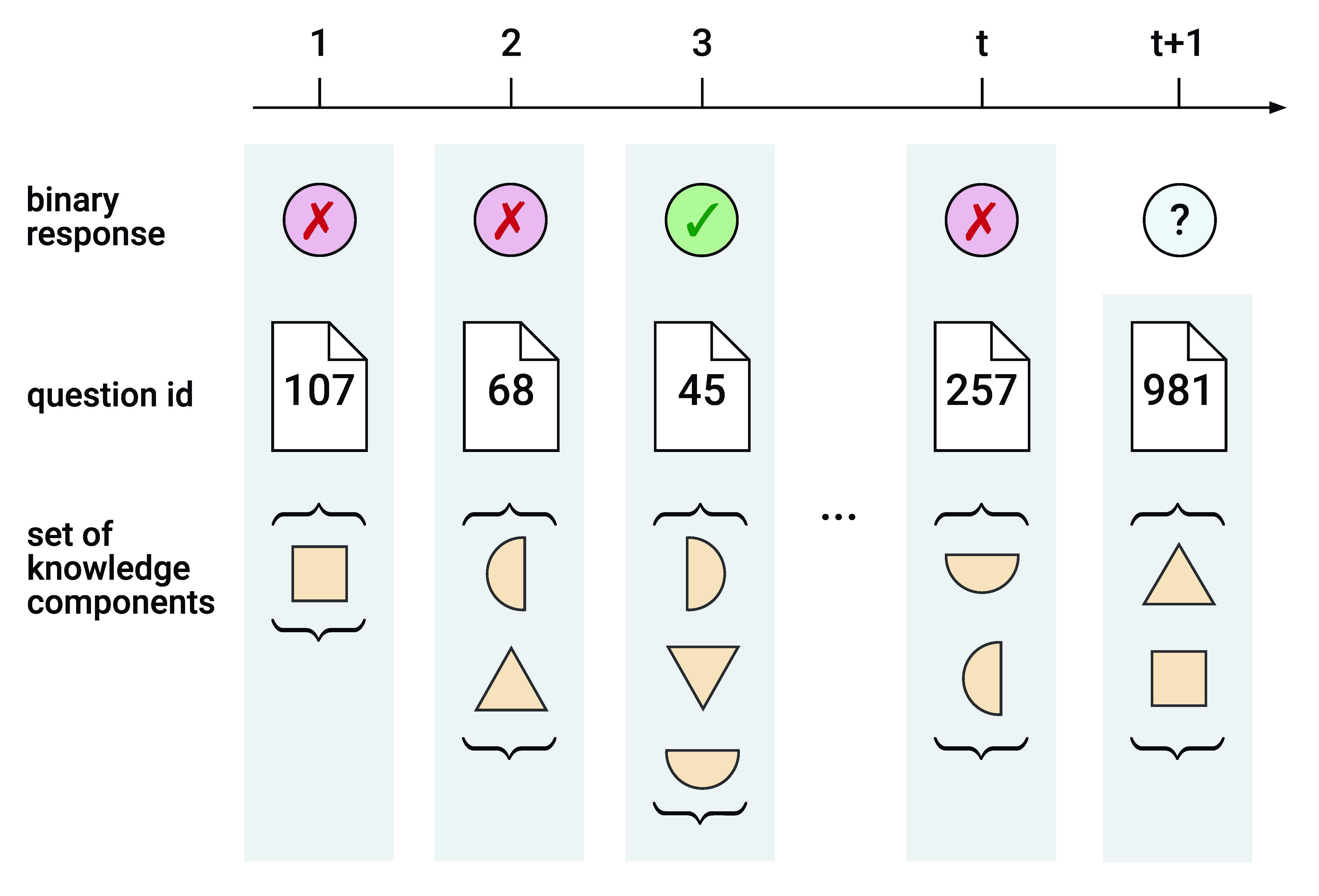
We study knowledge tracing as a supervised sequential learning task (cf. Gervet et al. 2020). That is, we predict the correctness of the next response by a student, given their learning history in the form of a sequence of interactions with a learning system. An interaction comprises all available information for a given time step. The prediction task can be formalized as follows. Consider a sequence of interactions of a student with a learning system. At any time \(1\leq t\leq T\), the student attempts to solve a question \(\rvq _t\in \gQ \) and their binary response \(\rvr _t \in \left \{ 0, 1 \right \}\) is observed, where \(\rvr _t = 1\) indicates a correct and \(\rvr _t = 0\) indicates an incorrect answer. Every question \(\rvq _t\) is associated with one or more knowledge components \(c\in \gC = \left \{ c_n \right \}_{n=1}^{\left |\gC \right |}\) given by \(\rvc (\rvq _t) \subseteq \gC \). In this context, knowledge components describe information and skills that are required to solve specific tasks or questions and that are part of a domain model. We summarize the sequence of interactions of a student by \(\rvy _{1:T}\) with \(\rvy _t = \left (\rvq _t, \rvc \left (\rvq _t\right ), \rvr _t \right )\). At time \(t\), the machine learning task is to predict the next response \(\rvr _{t + 1}\) given interactions \(\rvy _{1:t}\) and the next question \(\rvx _{t + 1} = \left (\rvq _{t + 1}, \rvc \left (\rvq _{t + 1}\right )\right )\).3 Figure 1 visualizes the setting.
In both Figure 1 and our description of the problem setting, we stress that knowledge components are inherently to be treated as sets. This is in contrast to well-published recent knowledge tracing approaches (e.g., Ghosh et al. 2020, Liu et al. 2022, Liu et al. 2023), which propose an interaction representation that stresses the effect of individual knowledge components on the learning task and that cannot properly handle multiple knowledge components per question. We refer to this representation as expanded representation (cf. Liu et al. 2022). In the expanded representation, each interaction involves a single question associated with a single knowledge component. Questions that are associated with multiple knowledge components in the original interaction sequence \(\rvy _{1:T}\) are therefore repeated, while knowledge components are distributed across the repetitions. Suppose an interaction \(\rvy _t\) is associated with multiple knowledge components \(|\rvc (\rvq _t)| \ge 2\). Its expanded representation is \(\tilde \rvy _t = (\rvq _t, \rvc \left (\rvq _t\right )_1, \rvr _t), \dots , (\rvq _t, \rvc \left (\rvq _t\right )_{|\rvc (\rvq _t)|}, \rvr _t)\). A direct consequence is an increase in sequence length by a factor depending on the average number of knowledge components per question. In prior work, models are trained to predict the next response based on this expanded representation. Without proper masking regarding the original interaction sequence, this introduces label leakage, i.e., parts of the expanded interactions have information about the response (the label at the current time step) due to the response being included in preceding interaction features of the expanded representation (e.g., Ghosh et al. 2020, Yin et al. 2023). Label leakage has been fixed in part by Liu et al. (2022). However, by fixing label leakage only for testing but not for training, the authors create a distribution shift between the data the model is trained on (which contains label leakage) and the data it is tested on (which does not). Hence, the model may learn to rely on label leakage during training, which then results in suboptimal predictions during inference. Empirically, we find that the performance of the expanded representation is noticeably worse for the EdNet dataset, which comes with a knowledge-component-to-question ratio larger than two (cf. Section 5.1).
4. Knowledge tracing set transformers
In this section, we propose knowledge tracing set transformers (KTSTs), a conceptually simple but effective model class for knowledge tracing. KTSTs closely follow prominent machine learning methods, use an intuitive set-based representation of student interactions, and minimize the need for domain-specific engineering. Specifically, KTSTs build upon a standard encoder-decoder architecture that is prevalent in transformer-based knowledge tracing approaches. KTSTs operate on principled representations of student interactions that are permutation invariant (cf. Zaheer et al. 2017) with respect to sets of knowledge components and specifically address the prevalent, yet flawed, expanded representation for interaction sequences in related work. To account for relative positional information, KTSTs include learnable ALiBi, a learnable variant of modification of attention matrices (cf. Press et al. 2021).
4.1. Transformer architecture for knowledge tracing
The deep learning architecture for KTSTs is based on the standard transformer architecture (Vaswani et al., 2017), including an encoder and a decoder, multiple layers with multi-head self-attention (MHSA) and cross-attention, residual connections (He et al., 2016), dropout (Srivastava et al., 2014), layer normalization (Ba et al., 2016), and feed-forward neural networks. Encoder-decoder architectures with cross-attention have previously been employed in transformer-based architectures for knowledge tracing (e.g., Yin et al. 2023, Im et al. 2023). The use of cross-attention from a question representation to an interaction representation was first proposed by Pandey and Karypis (2019). Choi et al. (2020) proposed encoding the interaction representation with self-attention, resulting in an encoder-decoder architecture. A key motivation and advantage of this architectural choice is the availability of complete interactions, including response information, where question and response do not have to be aligned in the architecture or via positional encoding alone. Instead of positional encodings, we employ a learnable modification of attention matrices (see Section 4.3); other differences are pointed out in the following. Overall, the architecture allows for efficient training with a single forward and backward pass per sequence.
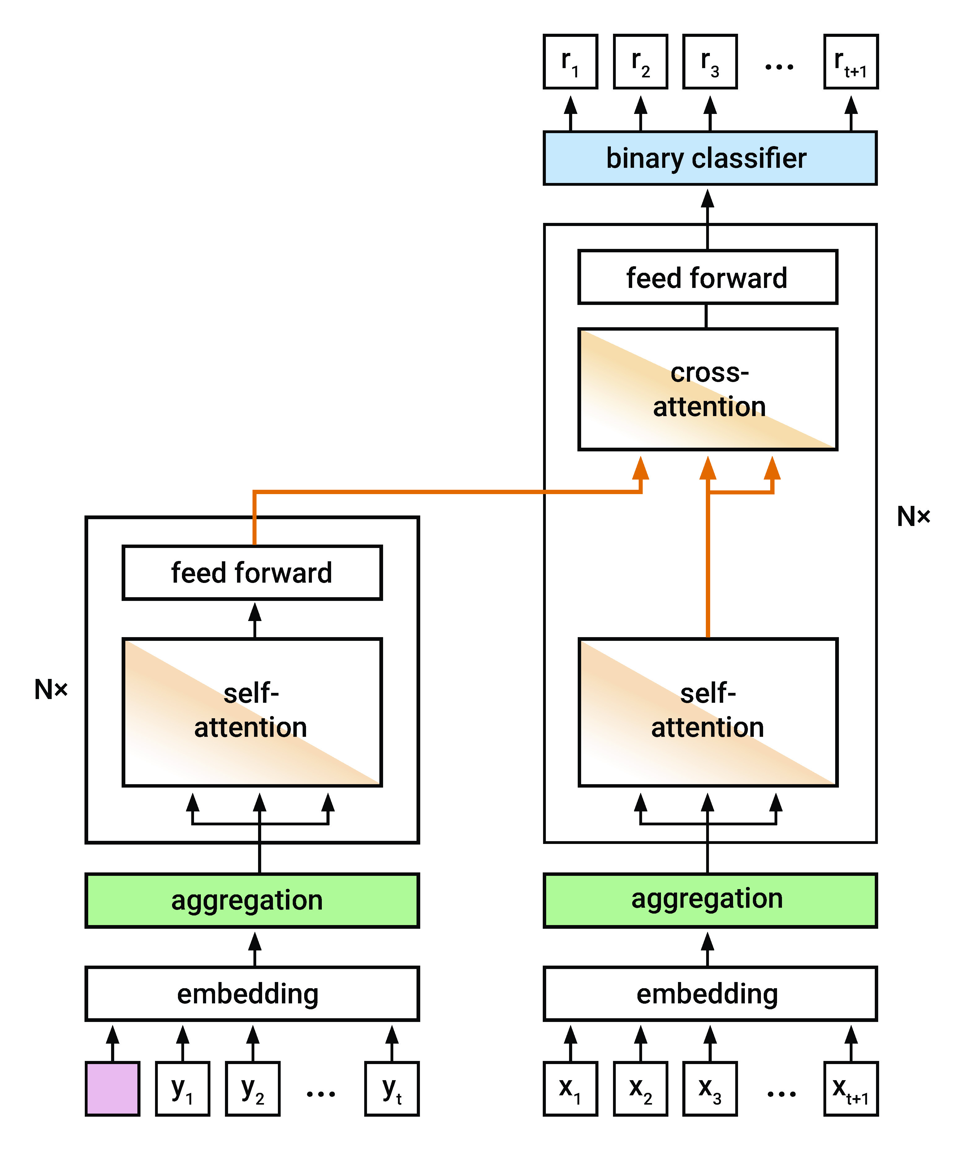
KTSTs operate on multiple discrete tokens per interaction \(\rvy _t\): a question \(\rvq _t\), its associated knowledge components \(\rvc \left (\rvq _t\right )\), and response \(\rvr _t\). We embed every token into a vector of size \(d\). Embeddings associated with the same time step are aggregated to form a joint interaction representation (respectively question representation; see Section 4.2). For each interaction, KTSTs estimate the probability of a correct response at the next time step, \(P(\rvr _{t+1}=1|\rvx _{t+1}, \rvy _{1:t})\). The representation of the question \(\rvx _{t+1}\) is used as query token in the decoder, attending to the learning history \(\rvy _{1:t}\) as processed by the encoder. We mask encoder and decoder appropriately: in both the encoder and the decoder, we use a triangular causal mask; in the encoder, the learning history is shifted by one time step and prepended by a learnable start token. Unlike standard transformers, we use the encoded \(\rvy _{1:t}\) only as value in the cross-attention layer, such that questions \(\rvx _{t+1}\) serve as both query and key within the cross-attention. For knowledge tracing, this adjustment has been proposed by Ghosh et al. (2020); within our architecture it is empirically supported by an ablation study (cf. Section 5.2). A binary classifier operating on the decoder’s output (concatenated with untransformed question representations via a global skip connection) yields the final probability estimates for a correct response. KTSTs are trained using standard binary cross-entropy loss between predicted and true responses.
See Figure 2 for a visualization of the model architecture. Differences from the standard transformer architecture are highlighted in color: The learnable start token is depicted in pink. The components depicted in green point to KTSTs interaction aggregation methods, which we introduce in Section 4.2. The components highlighted in orange refer to deviations from the standard attention mechanism, namely differences in cross-attention as explained above, as well as the use of learnable ALiBi, which we introduce in Section 4.3. The binary classifier is highlighted in blue.
4.2. Set-based interaction representations
For KTSTs, we study interaction representations that address the set-based nature of interaction features. The representations use standard machine learning paradigms for feature extraction and are domain-agnostic. This is especially in contrast with the expanded representation which is prevalent in recent publications (e.g., Ghosh et al. 2020, Liu et al. 2023, Liu et al. 2022). Besides the fundamental issues addressed in Section 3, the expanded representation violates permutation invariance (which we formally introduce below), as the order of knowledge components influences both the transformation within the model as well as final probability scores.4
Since our primary concern is data from educational learning settings that involve multiple knowledge components per student interaction, for KTSTs we study three different aggregation methods for student interactions, resulting in: mean embeddings, unique set embeddings, and multi-head self-attention (MHSA) embeddings.
Within KTSTs, the elements of every interaction \(\rvy _t = \left (\rvq _t, \rvc \left (\rvq _t\right ), \rvr _t \right )\) are embedded separately and aggregated to form joint representations that are used as inputs to the transformer architecture.5 We require the aggregation function for interaction tuples \(\rvy _t\) (and question tuples \(\rvx _t\)) to be permutation invariant (cf. Zaheer et al. 2017) to the ordering of knowledge components \(\rvc \left (\rvq _t\right )\) associated with question \(\rvq _t\). Permutation invariance is a desirable property of functions operating on sets. Formally, consider a question \(\rvq \) with \(k\) associated knowledge components and let \(\rvn = \rvn (\rvq )\) be their corresponding indices. Let \(\pi \) denote a permutation of a \(k\)-tuple of integers \(1\) through \(k\). For the aggregation function \(\phi \left (\rvx \right )\) to be permutation invariant with respect to the ordering of knowledge components, it must hold that
for any permutation \(\pi \). This definition also applies to the ordering of knowledge components in representation \(\phi (\rvy )\).
Consider the following three permutation invariant aggregation functions: First, the mean operation satisfies permutation invariance (cf. Zaheer et al. 2017). Second, a function that assigns an integer to any unique set is also permutation invariant (for illustration, consider that the function orders the set first and only then assigns an integer to the ordered tuple, in which case ordering yields permutation invariance). Third, unmasked multi-head self-attention with standard scaled dot-product attention applied to a set of tokens without positional encoding yields permutation invariant representations per token, since attention weights are indifferent to the ordering of tokens (this property is usually referred to as permutation equivariance; for a formal proof compare, for example, Girgis et al. 2022).
Let \(\rve _{*} \in \sR ^d\) denote embedding vectors and let \(\oplus \) denote element-wise addition. For KTSTs, we propose using the above aggregation methods to embed student interactions, resulting in three mutually exclusive interaction embeddings \(\rve _{\rvy }\) that adhere to permutation invariant aggregation. Associated question embeddings \(\rve _{\rvx }\) (that omit response embeddings \(\rve _\rvr \)) are computed analogously.
First, for mean embeddings we assign unique embedding vectors \(\rve _c\) to each knowledge component in \(\rvc (\rvq )\) and compute their mean. Final interaction embeddings are the result of element-wise addition with question \(\rve _\rvq \) and response embedding \(\rve _\rvr \):
Second, for unique set embeddings we assign a unique embedding vector \(\rve _{\unique (\left \{c | c \in \rvc (\rvq )\right \})}\) to each unique set of knowledge components. The final interaction embedding is computed as above:
Third, for MHSA embeddings we pass a sequence containing a query token, the question embedding \(\rve _\rvq \) and embedding vectors \(\rve _c\) for knowledge components in \(\rvc (\rvq )\) through (possibly multiple layers) of unmasked multi-head self-attention \(\MHSA \). The final interaction embedding equals the element-wise addition of transformed query token and response embedding \(\rve _\rvr \):
All three interaction embeddings are straightforward and domain-agnostic. Specifically, while our model uses knowledge components as provided in the data, it is oblivious to what these features describe. This is in contrast to the embeddings by Ghosh et al. (2020) and Liu et al. (2023), who explicitly model the interactions according to how knowledge components might change the difficulty of a question.
Mean embeddings allow the models to attribute student performance to individual knowledge components, while we conjecture interaction effects to be more difficult to learn. Unique set embeddings naturally account for interactions. However, we argue that it becomes increasingly difficult to attribute responses to individual knowledge components, as the approach results in a (theoretically) exponential increase in the number of embeddings, each of which has only a few occurrences. In principle, MHSA embeddings involve the most general and powerful aggregation of knowledge components, accounting for both individual and interaction effects. Importantly, MHSA embeddings are designed to readily incorporate an arbitrary number of additional, potentially more complex features associated with an interaction.
Empirically, we observe that for knowledge tracing tasks with small knowledge-component-to-question ratios, simple aggregations like mean embeddings and unique set embeddings of knowledge components seem to work equally well, while MHSA embeddings are difficult to optimize and result in overfitting. We conjecture that MHSA embeddings perform better in more complicated settings with large data, as we see comparatively better performance for larger datasets with many knowledge components, such as the EdNet dataset (see Section 5.1). This conjecture is supported by experiments on synthetic data, where we experiment with varying knowledge-component-to-question ratios and dataset sizes (see Section 5.3). We consider all three interaction embeddings to have their respective use cases. Practitioners should decide on an appropriate interaction embedding depending on their specific setting.
In contrast to the above representations, interaction representations proposed in related work are often domain-specific and unnecessarily complex. Specifically, we consider all three interaction embeddings proposed for KTSTs conceptually simpler than domain-specific Rasch embeddings used in Ghosh et al. (2020) and other recent knowledge tracing models (e.g., Liu et al. 2023, Yin et al. 2023). In short, Rasch embeddings prescribe that questions are represented as \(\rve _{\rvx } = \rve _c \oplus (\rve _q \cdot \rvv _c)\), i.e., as the addition of two embeddings related to the same knowledge component \(\rve _c \in \sR ^d\) and \(\rvv _c \in \sR ^d\), where the latter is supposed to capture knowledge-component-specific variations and is scaled by \(\rve _q \in \sR \), a scalar embedding of questions that “controls how far this question deviates from the [knowledge component] it covers” (Ghosh et al., 2020). Interactions are represented analogously with knowledge-component-response embeddings and knowledge-component-response variation vectors. Given these design choices, Rasch embeddings require the flawed expanded representation. Given that KTSTs set a new state-of-the-art (see Section 5.1), we provide empirical evidence that straightforward set-based representations are sufficient to capture domain-specific information within knowledge tracing tasks.
4.3. Learnable modification of attention matrices
In transformer architectures, positional information is usually conveyed by including positional embeddings or by modifying attention matrices (Dufter et al., 2022). For KTSTs, we propose a multi-head attention mechanism with learnable exponential decay applied to attention weights at previous time steps to account for the sequential nature of the learning task, following Press et al. (2021). Exponential decay applied to attention weights reduces attention scores based on relative distances of key tokens to the query token. Similar attention functions have, for example, been investigated for knowledge tracing tasks by Ghosh et al. (2020) and Im et al. (2023).
Let \(\alpha _{t,t-\tau } \in \left [0, 1\right ]\) denote the attention weights calculated in a single head for query \(q_t \in \sR ^d\) and key \(k_{t-\tau } \in \sR ^d\) at time steps \(t\) and \(t - \tau \), respectively, with \(0\leq \tau \leq t-1\). Assuming causal masking, where attention weights for \(\alpha _{t,>t}\) are set to \(0\), the standard scaled dot product attention weight between two tokens, as introduced in Vaswani et al. (2017), results from the application of a softmax
to (unbounded) attention scores \(e_{t,t-\tau }\). Abstracting from in-projections, \(e_{t,t-\tau }\) is given by
In KTSTs’ attention, we subtract a non-negative value \(\tau \theta \geq 0\) from attention scores \(e_{t,t-\tau }\):
Here, \(\theta \) is a learnable parameter per attention head, which we restrict to be positive via application of the softplus function (Dugas et al., 2000, Glorot et al., 2011). We initialize effective values of \(\theta \) according to the geometric series as prescribed by Press et al. (2021) for ALiBi (attention with linear biases, where linearity refers to attention scores). Hence, for models with four attention heads, \(\theta \) is initialized with \(\frac {1}{2^2}, \frac {1}{2^4}, \frac {1}{2^6}\) and \(\frac {1}{2^8}\), respectively, while models with eight heads give rise to the initialization \(\frac {1}{2^1}, \frac {1}{2^2}, \dots , \frac {1}{2^8}\).
The initialization introduces an inductive bias at the beginning of the training process, where interactions with a higher relative distance are assigned a lower weight in the attention mechanism. In general, KTSTs’ attention mechanism results in attention weights that are exponentially decayed. For \(\theta = 0\), we have \(\alpha _{t,t-\tau }^{\KTST } = \alpha _{t,t-\tau }^{\standard }\), whereas for large values of \(\theta \), we have \(\alpha _{t,t}^{\KTST } \approx 1\) and \(\alpha _{t,<t}^{\KTST } \approx 0\). In the absence of positional encoding, this results in an attention function that interpolates between attention on a set for \(\theta \approx 0\) and soft sliding windows (which are possibly very narrow) applied to interactions at time steps \(<\!\!t\) for large \(\theta \). Im et al. (2023) associate ALiBi with students’ forgetting behavior. However, performance improvements when using ALiBi may be related to employing relative rather than absolute positional encoding. Empirically, the proposed handling of positional information within the attention mechanism performs best for KTSTs (see an ablation study in Section 5.2).
5. Experiments
In this section, we empirically evaluate the proposed knowledge tracing set transformers on a benchmark with standardized tasks, preprocessing, data splits, and fixed test sets for various educational datasets (pyKT, Liu et al. 2022). We thus provide evidence that KTSTs set a new state-of-the-art for the knowledge tracing prediction task. Furthermore, we verify the encoder-decoder architecture as well as the proposed learnable modification of attention matrices used in KTSTs in an ablation study. We additionally experiment with synthetic data, generated according to classic multidimensional item response theory (MIRT, Reckase 2009), to study the performance of the proposed set-based interaction representations in knowledge tracing settings with high knowledge-component-to-question ratios.
5.1. State-of-the-art benchmark results
We evaluate KTSTs on the pyKT benchmark (Liu et al., 2022). In accordance with standard practice in knowledge tracing, we report AUC and accuracy values. In summary, we experiment on eight publicly available datasets: EdNet (Choi et al., 2020), Algebra2005 (AL2005) (Stamper et al., 2010a), ASSISTments2009 (AS2009) (Feng et al., 2009), NeurIPS34 (Wang et al., 2020), Bridge2006 (BD2006) (Stamper et al., 2010b), Statics2011 (Bier, 2011), ASSISTments2015 (AS2015), and POJ (Pandey and Srivastava, 2020).6 Preprocessing following Liu et al. (2022) omits features available in some of the original datasets; the EdNet dataset is sub-sampled. As indicated in Section 4.2, KTSTs with MHSA embeddings could readily leverage additional features. For a fair comparison, we restrict our experiments to pyKT’s feature set. We compare against the following baselines: DKT (Piech et al., 2015), DKVMN (Zhang et al., 2017), DKT+ (Yeung and Yeung, 2018), DeepIRT (Yeung, 2019), DKT-F (Nagatani et al., 2019), GKT (Nakagawa et al., 2019), KQN (Lee and Yeung, 2019), SAKT (Pandey and Karypis, 2019), SKVMN (Abdelrahman and Wang, 2019), AKT (Ghosh et al., 2020), qDKT (Sonkar et al., 2020), SAINT (Choi et al., 2020), ATKT (Guo et al., 2021), HawkesKT (Wang et al., 2021), IEKT (Long et al., 2021), LPKT (Shen et al., 2021), DIMKT (Shen et al., 2022), AT-DKT (Liu et al., 2023), DTransformer (Yin et al., 2023), FoLiBiKT (Im et al., 2023), QIKT (Chen et al., 2023), and simpleKT (Liu et al., 2023). Notable baselines are discussed in related work in Section 2, in the problem setting in Section 3, as well as in contrast to our contribution in Section 4.
Models are trained on sequences of at most 200 consecutive interactions each and tested on entire interaction sequences of students in the test set.7 All baseline results are reproduced by us using the model implementations and hyperparameters provided by Liu et al. (2022). During hyperparameter optimization, a budget of 200 runs has been granted for each combination of baseline and data fold. We refer to Liu et al. (2022) for more details on search spaces and the tuning procedure. Hyperparameters of KTST models are tuned according to a tree-structured Parzen estimator (Bergstra et al., 2011, Akiba et al., 2019), with a budget of 100 runs for each data fold. Model selection is performed via a 5-fold cross-validation, using AUC as the selection criterion. Details on the hyperparameter optimization can be found in Appendix A.
Table 1 (AUC) and 2 (accuracy) show mean performance and standard deviations for KTSTs for the most important datasets and baselines. Due to lack of space, full results are provided in Appendix C, which include experiments regarding datasets Statics2011, AS2015, and POJ and baselines DeepIRT, DKT-F, KQN, qDKT, ATKT, and AT-DKT. KTST (mean), KTST (unique), and KTST (MHSA) refer to KTST architectures with mean embeddings, unique set embeddings, and MHSA embeddings, respectively. For datasets with a knowledge-component-to-question ratio of \(1.0\) (Statics2011, AS2015, POJ), or approximately \(1.0\) (NeurIPS34, BD2006), we only provide KTST (mean) results, as KTST (unique) results are expected to be identical and KTST (MHSA) embeddings are expected to be nearly identical, but inefficient in these settings. KTST models achieve state-of-the-art AUC results on all datasets except Statics2011. For accuracy, the results are similar. Comparing KTST (mean) to all baselines, its performance improvements were statistically confirmed using one-sided paired t-tests and the Holm-Bonferroni correction (\(\alpha =0.01\)): the null hypothesis was rejected in favor of KTST in almost all comparisons.
| EdNet | AL2005 | AS2009 | NeurIPS34 | BD2006 | |
|---|---|---|---|---|---|
| DKT | 0.6108 \(\pm \) 0.0017\(\ast \) | 0.8137 \(\pm \) 0.0018\(\ast \) | 0.7532 \(\pm \) 0.0012\(\ast \) | 0.7682 \(\pm \) 0.0006\(\ast \) | 0.8011 \(\pm \) 0.0005\(\ast \) |
| DKVMN | 0.6158 \(\pm \) 0.0020\(\ast \) | 0.8060 \(\pm \) 0.0016\(\ast \) | 0.7461 \(\pm \) 0.0010\(\ast \) | 0.7675 \(\pm \) 0.0004\(\ast \) | 0.7980 \(\pm \) 0.0014\(\ast \) |
| DKT+ | 0.6156 \(\pm \) 0.0018\(\ast \) | 0.8142 \(\pm \) 0.0004\(\ast \) | 0.7536 \(\pm \) 0.0016\(\ast \) | 0.7688 \(\pm \) 0.0002\(\ast \) | 0.8012 \(\pm \) 0.0006\(\ast \) |
| GKT | 0.6213 \(\pm \) 0.0024\(\ast \) | 0.8085 \(\pm \) 0.0018\(\ast \) | 0.7422 \(\pm \) 0.0028\(\ast \) | 0.7650 \(\pm \) 0.0071\(\ast \) | 0.8043 \(\pm \) 0.0013\(\ast \) |
| SAKT | 0.6074 \(\pm \) 0.0013\(\ast \) | 0.7887 \(\pm \) 0.0042\(\ast \) | 0.7245 \(\pm \) 0.0009\(\ast \) | 0.7507 \(\pm \) 0.0011\(\ast \) | 0.7732 \(\pm \) 0.0010\(\ast \) |
| SKVMN | 0.6230 \(\pm \) 0.0045\(\ast \) | 0.7461 \(\pm \) 0.0033\(\ast \) | 0.7326 \(\pm \) 0.0016\(\ast \) | 0.7502 \(\pm \) 0.0012\(\ast \) | 0.7286 \(\pm \) 0.0046\(\ast \) |
| AKT | 0.6705 \(\pm \) 0.0024\(\ast \) | 0.8298 \(\pm \) 0.0017\(\ast \) | 0.7840 \(\pm \) 0.0016\(\ast \) | 0.8030 \(\pm \) 0.0003\(\ast \) | 0.8204 \(\pm \) 0.0006\(\ast \) |
| SAINT | 0.6598 \(\pm \) 0.0023\(\ast \) | 0.7767 \(\pm \) 0.0018\(\ast \) | 0.6918 \(\pm \) 0.0036\(\ast \) | 0.7866 \(\pm \) 0.0023\(\ast \) | 0.7762 \(\pm \) 0.0025\(\ast \) |
| HawkesKT | 0.6815 \(\pm \) 0.0041\(\ast \) | 0.8207 \(\pm \) 0.0021\(\ast \) | 0.7224 \(\pm \) 0.0006\(\ast \) | 0.7757 \(\pm \) 0.0014\(\ast \) | 0.8067 \(\pm \) 0.0011\(\ast \) |
| IEKT | 0.7301 \(\pm \) 0.0012\(\ast \) | 0.8403 \(\pm \) 0.0019\(\ast \) | 0.7832 \(\pm \) 0.0021\(\ast \) | 0.8039 \(\pm \) 0.0003\(\ast \) | 0.8116 \(\pm \) 0.0013\(\ast \) |
| LPKT | 0.7340 \(\pm \) 0.0007\(\ast \) | 0.8239 \(\pm \) 0.0008\(\ast \) | 0.7811 \(\pm \) 0.0019\(\ast \) | 0.7940 \(\pm \) 0.0012\(\ast \) | 0.8039 \(\pm \) 0.0004\(\ast \) |
| DIMKT | 0.6748 \(\pm \) 0.0030\(\ast \) | 0.8276 \(\pm \) 0.0007\(\ast \) | 0.7717 \(\pm \) 0.0010\(\ast \) | 0.8022 \(\pm \) 0.0009\(\ast \) | 0.8166 \(\pm \) 0.0007\(\ast \) |
| DTransformer | 0.6719 \(\pm \) 0.0037\(\ast \) | 0.8189 \(\pm \) 0.0024\(\ast \) | 0.7718 \(\pm \) 0.0021\(\ast \) | 0.7990 \(\pm \) 0.0006\(\ast \) | 0.8083 \(\pm \) 0.0006\(\ast \) |
| FoLiBiKT | 0.6721 \(\pm \) 0.0018\(\ast \) | 0.8307 \(\pm \) 0.0005\(\ast \) | 0.7828 \(\pm \) 0.0016\(\ast \) | 0.8028 \(\pm \) 0.0005\(\ast \) | 0.8203 \(\pm \) 0.0015\(\ast \) |
| QIKT | 0.7260 \(\pm \) 0.0013\(\ast \) | 0.8408 \(\pm \) 0.0008\(\ast \) | 0.7877 \(\pm \) 0.0019\(\ast \) | 0.8041 \(\pm \) 0.0008\(\ast \) | 0.8094 \(\pm \) 0.0008\(\ast \) |
| simpleKT | 0.6593 \(\pm \) 0.0041\(\ast \) | 0.8246 \(\pm \) 0.0012\(\ast \) | 0.7745 \(\pm \) 0.0021\(\ast \) | 0.8035 \(\pm \) 0.0002\(\ast \) | 0.8159 \(\pm \) 0.0005\(\ast \) |
| KTST (mean) | 0.7394 \(\pm \) 0.0002 \(\:\) | 0.8522 \(\pm \) 0.0004 \(\:\) | 0.7993 \(\pm \) 0.0012 \(\:\) | 0.8071 \(\pm \) 0.0000 \(\:\) | 0.8264 \(\pm \) 0.0004 \(\:\) |
| KTST (unique) | 0.7355 \(\pm \) 0.0008 \(\:\) | 0.8529 \(\pm \) 0.0009 \(\:\) | 0.7989 \(\pm \) 0.0014 \(\:\) | — | — |
| KTST (MHSA) | 0.7389 \(\pm \) 0.0009 \(\:\) | 0.8288 \(\pm \) 0.0009 \(\:\) | 0.7871 \(\pm \) 0.0022 \(\:\) | — | — |
| EdNet | AL2005 | AS2009 | NeurIPS34 | BD2006 | |
|---|---|---|---|---|---|
| DKT | 0.6420 \(\pm \) 0.0023\(\ast \) | 0.8094 \(\pm \) 0.0010\(\ast \) | 0.7241 \(\pm \) 0.0012\(\ast \) | 0.7024 \(\pm \) 0.0008\(\ast \) | 0.8551 \(\pm \) 0.0003\(\ast \) |
| DKVMN | 0.6446 \(\pm \) 0.0030\(\ast \) | 0.8031 \(\pm \) 0.0008\(\ast \) | 0.7194 \(\pm \) 0.0006\(\ast \) | 0.7020 \(\pm \) 0.0004\(\ast \) | 0.8545 \(\pm \) 0.0003\(\ast \) |
| DKT+ | 0.6517 \(\pm \) 0.0057\(\ast \) | 0.8093 \(\pm \) 0.0004\(\ast \) | 0.7241 \(\pm \) 0.0013\(\ast \) | 0.7034 \(\pm \) 0.0005\(\ast \) | 0.8551 \(\pm \) 0.0002\(\ast \) |
| GKT | 0.6639 \(\pm \) 0.0050\(\ast \) | 0.8086 \(\pm \) 0.0008\(\ast \) | 0.7158 \(\pm \) 0.0016\(\ast \) | 0.6956 \(\pm \) 0.0103\(\ast \) | 0.8553 \(\pm \) 0.0003\(\ast \) |
| SAKT | 0.6392 \(\pm \) 0.0039\(\ast \) | 0.7959 \(\pm \) 0.0018\(\ast \) | 0.7071 \(\pm \) 0.0016\(\ast \) | 0.6870 \(\pm \) 0.0010\(\ast \) | 0.8456 \(\pm \) 0.0006\(\ast \) |
| SKVMN | 0.6606 \(\pm \) 0.0090\(\ast \) | 0.7821 \(\pm \) 0.0032\(\ast \) | 0.7160 \(\pm \) 0.0010\(\ast \) | 0.6874 \(\pm \) 0.0010\(\ast \) | 0.8408 \(\pm \) 0.0005\(\ast \) |
| AKT | 0.6645 \(\pm \) 0.0035\(\ast \) | 0.8125 \(\pm \) 0.0016\(\ast \) | 0.7383 \(\pm \) 0.0020\(\ast \) | 0.7317 \(\pm \) 0.0005\(\ast \) | 0.8586 \(\pm \) 0.0005\(\ast \) |
| SAINT | 0.6511 \(\pm \) 0.0039\(\ast \) | 0.7789 \(\pm \) 0.0030\(\ast \) | 0.6885 \(\pm \) 0.0044\(\ast \) | 0.7172 \(\pm \) 0.0025\(\ast \) | 0.8374 \(\pm \) 0.0108\(\ast \) |
| HawkesKT | 0.6905 \(\pm \) 0.0025\(\ast \) | 0.8112 \(\pm \) 0.0012\(\ast \) | 0.7045 \(\pm \) 0.0008\(\ast \) | 0.7102 \(\pm \) 0.0013\(\ast \) | 0.8559 \(\pm \) 0.0005\(\ast \) |
| IEKT | 0.7106 \(\pm \) 0.0018\(\ast \) | 0.8228 \(\pm \) 0.0008\(\ast \) | 0.7336 \(\pm \) 0.0027\(\ast \) | 0.7327 \(\pm \) 0.0001\(\ast \) | 0.8556 \(\pm \) 0.0009\(\ast \) |
| LPKT | 0.7128 \(\pm \) 0.0004\(\ast \) | 0.8129 \(\pm \) 0.0008\(\ast \) | 0.7356 \(\pm \) 0.0011\(\ast \) | 0.7179 \(\pm \) 0.0033\(\ast \) | 0.8538 \(\pm \) 0.0002\(\ast \) |
| DIMKT | 0.6700 \(\pm \) 0.0038\(\ast \) | 0.8106 \(\pm \) 0.0004\(\ast \) | 0.7354 \(\pm \) 0.0019\(\ast \) | 0.7309 \(\pm \) 0.0005\(\ast \) | 0.8578 \(\pm \) 0.0004\(\ast \) |
| DTransformer | 0.6656 \(\pm \) 0.0032\(\ast \) | 0.8054 \(\pm \) 0.0007\(\ast \) | 0.7284 \(\pm \) 0.0007\(\ast \) | 0.7290 \(\pm \) 0.0012\(\ast \) | 0.8556 \(\pm \) 0.0006\(\ast \) |
| FoLiBiKT | 0.6666 \(\pm \) 0.0028\(\ast \) | 0.8127 \(\pm \) 0.0012\(\ast \) | 0.7391 \(\pm \) 0.0013\(\ast \) | 0.7319 \(\pm \) 0.0005\(\ast \) | 0.8583 \(\pm \) 0.0006\(\ast \) |
| QIKT | 0.7077 \(\pm \) 0.0014\(\ast \) | 0.8220 \(\pm \) 0.0007\(\ast \) | 0.7382 \(\pm \) 0.0008\(\ast \) | 0.7326 \(\pm \) 0.0008\(\ast \) | 0.8537 \(\pm \) 0.0005\(\ast \) |
| simpleKT | 0.6565 \(\pm \) 0.0029\(\ast \) | 0.8081 \(\pm \) 0.0010\(\ast \) | 0.7319 \(\pm \) 0.0019\(\ast \) | 0.7327 \(\pm \) 0.0003\(\ast \) | 0.8579 \(\pm \) 0.0002\(\ast \) |
| KTST (mean) | 0.7154 \(\pm \) 0.0011 \(\:\) | 0.8287 \(\pm \) 0.0005 \(\:\) | 0.7490 \(\pm \) 0.0013 \(\:\) | 0.7356 \(\pm \) 0.0003 \(\:\) | 0.8608 \(\pm \) 0.0005 \(\:\) |
| KTST (unique) | 0.7131 \(\pm \) 0.0017 \(\:\) | 0.8291 \(\pm \) 0.0008 \(\:\) | 0.7489 \(\pm \) 0.0011 \(\:\) | — | — |
| KTST (MHSA) | 0.7152 \(\pm \) 0.0011 \(\:\) | 0.8166 \(\pm \) 0.0012 \(\:\) | 0.7415 \(\pm \) 0.0014 \(\:\) | — | — |
The principled and permutation invariant aggregation of knowledge components is one of the strengths of KTSTs. Compared to baselines using the flawed expanded representation, we thus expect the largest gains in performance for the datasets EdNet, AL2005, and AS2009, with an average knowledge-components-per-question ratio of \(2.24\), \(1.36\), and \(1.19\), respectively. The results confirm our hypothesis, with differences being most pronounced on EdNet, where IEKT, LPKT, and QIKT are the only baselines that are in the same ballpark as KTST results. Notably, all three models also employ set-based interaction representations. KTST (mean) generally performs well. Unique set embeddings turn out to be more suited for small component-to-question ratios, as they seem to incur a penalty for higher knowledge-component-to-question ratios, whereas KTST (MHSA)’s performance is only competitive on EdNet. We conjecture that KTST (MHSA)’s modeling capacity might be too high for simpler knowledge tracing tasks, resulting in more difficult optimization. We support this conjecture in experiments on synthetic data in Section 5.3.
5.2. Ablation study of attention mechanism
| Attention mechanism | AUC | ACC |
|---|---|---|
| Standard MHA + PE (q\(\neq \)k) | 0.7744 \(\pm \) 0.0014\(\ast \) | 0.7307 \(\pm \) 0.0015\(\ast \) |
| AKT (q\(=\)k) | 0.7958 \(\pm \) 0.0011\(\ast \) | 0.7464 \(\pm \) 0.0009\(\ast \) |
| ALiBi (q\(\neq \)k) | 0.7953 \(\pm \) 0.0018\(\ast \) | 0.7456 \(\pm \) 0.0021\(\ast \) |
| ALiBi (q\(=\)k) | 0.7978 \(\pm \) 0.0010\(\ast \) | 0.7479 \(\pm \) 0.0007 \(\:\) |
| Learnable ALiBi (q\(\neq \)k) | 0.7976 \(\pm \) 0.0013\(\ast \) | 0.7476 \(\pm \) 0.0012 \(\:\) |
| Learnable ALiBi (q\(=\)k) decoder-only | 0.7977 \(\pm \) 0.0011\(\ast \) | 0.7473 \(\pm \) 0.0007\(\ast \) |
| Learnable ALiBi (q\(=\)k) | 0.7993 \(\pm \) 0.0012 \(\:\) | 0.7490 \(\pm \) 0.0013 \(\:\) |
In an ablation study, we evaluate the performance of different attention mechanisms in KTSTs. Specifically, we address different ways of handling positional information, including positional embeddings and mechanisms that modify attention matrices. Table 3 provides results on the AS2009 dataset, where we compare KTST (mean) with four different types of attention mechanisms: Standard MHA + PE refers to standard multi-head attention with positional embeddings, AKT refers to the attention mechanism proposed in Ghosh et al. (2020), ALiBi refers to the attention mechanism proposed in Press et al. (2021) for language models, and Learnable ALiBi refers to the learnable modification of attention matrices that we propose to use in KTSTs (Section 4.3). Additionally, entries \(q=k\) and \(q\neq k\) refer to whether the query is set to equal the key in the cross-attention. In KTSTs, we set \(q=k\) following related work (see Section 4.1). Decoder-only refers to an architecture without an encoder, as suggested in Zhan et al. (2024). This corresponds to a KTST architecture with the number of encoder layers set to \(0\). Specifically, this implies that we still perform cross-attention, but that cross-attention is performed on the raw interaction representations – that is, the interaction embedding is not passed through any subsequent self-attention layers of an encoder. We report the mean and standard deviation of test results based on training with 5-fold validation.
We observe that learnable ALiBi achieves the best performance and that using the same token for both key and query in the cross-attention is favorable. Improvements are statistically confirmed using one-sided paired t-tests and the Holm-Bonferroni correction: the null hypothesis was rejected in favor of Learnable ALiBi (q=k) in almost all comparisons. The findings partially explain the good performance of KTSTs regarding the pyKT benchmark in Section 5.1 and support our design choices for KTSTs’ attention mechanism: a learnable attention function that interpolates between attention on a set of tokens and soft sliding windows over a sequence of tokens.
While a comparison of different interaction embeddings is not the objective of the ablation study, we can observe the following: Mean embeddings with AKT’s attention mechanism improve over the AKT baseline with Rasch embeddings on AS2009 (AUC: \(0.7958 \pm 0.0011\) over \(0.7840 \pm 0.0016\); Accuracy: \(0.7464 \pm 0.0009\) over \(0.7383 \pm 0.0020\)). We read this as empirical evidence against the expanded representation (which is implicitly required by the Rasch embedding).
5.3. Study of set-based interaction representations in KTSTs
In this section, we report on synthetic data generated according to classic multidimensional item response theory (MIRT, Reckase 2009), where we train on sequences with varying numbers of knowledge components per question. We thereby study the effect of different aggregation methods for interaction representations within KTSTs. Specifically, we sample interactions from a compensatory multidimensional 3PL model (Reckase, 2009). For question \(i\) and learner \(j\), the probability of a correct response is given by
where \(c_i\) denotes the probability of guessing a correct response for question \(i\), \(b_i \in \sR ^k\) and \(\theta _j \in \sR ^k\) are vectors with latent difficulties and student skills per knowledge component, respectively, and \(k\) indicates the total number of knowledge components. A randomly sampled multi-hot vector \(\tilde {a}_i \in \left \{0, 1\right \}^k\) assigns either two, three, or four knowledge components to questions, respectively, according to the experimental setting; we use normalized \(a_i = \tilde {a}_i / || \tilde {a}_i ||_1\) within the simulation. We set \(c_i=0.1\) for all questions and sample both \(b_i\) and \(\theta _i\) from an isotropic multivariate normal distribution (with variances equal to \(1.0\) and means \(0.0\) and \(-2.0\), respectively). If a student interacts with a knowledge component, we increase their respective latent skill by a constant factor.
Setting the number of questions to 1,000 and the total number of components to 50, we simulate \(100\) interactions per student and train KTST models on different sample sizes. For each configuration, we train 10 models and report test results on 5,000 interaction sequences. Hyperparameters are set according to preliminary experiments and are not tuned within each training run. We validated that the chosen hyperparameters worked for all models; all models outperform a naive baseline, predicting responses based on the average correctness rate per time step. Figure 3 visualizes the results of the experiment.
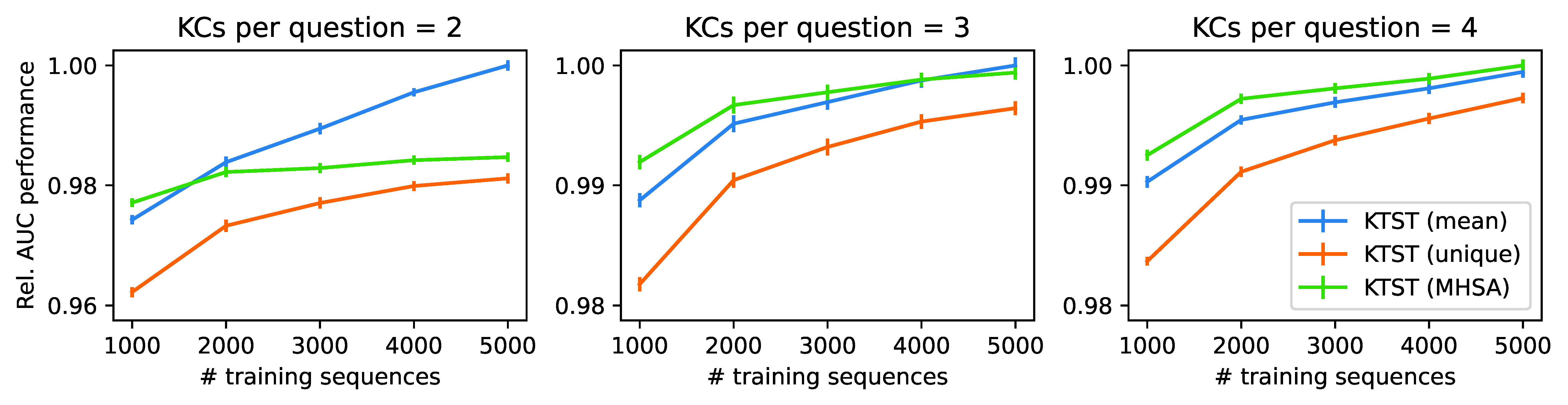
As expected, unique set embeddings perform worst throughout all experiments and data regimes. Regarding mean embeddings and MHSA embeddings, the experiments indicate a regime shift, where mean embeddings perform best on data with two knowledge components per question, while MHSA embeddings perform best on four knowledge components per question. Regarding three knowledge components per question, MHSA outperforms mean embeddings on smaller sample sizes, while mean embeddings seem to be better for 5,000 training sequences. Relatively, mean embeddings seem to benefit most from larger training data. Even though the generated data is simplistic and does not account for more complex effects which potentially arise in intelligent tutoring systems, the results on synthetic data support our conjecture that MHSA embeddings might constitute a good fit for more complex educational data than is available in current benchmark tasks.
6. Conclusion
In this paper, we proposed knowledge tracing set transformers (KTSTs), a straightforward, yet principled and performant model class for knowledge tracing prediction tasks. KTSTs are conceptually simple and easy to implement because they closely follow prominent machine learning methods and minimize the need for domain-specific engineering.
Specifically, KTSTs build upon a standard encoder-decoder architecture that is prevalent in transformer-based knowledge tracing approaches. Further, we studied three set-based representations of student interactions which are permutation invariant with respect to sets of knowledge components and which specifically address the prevalent, yet flawed, expanded representation for interaction sequences in related work. While mean embeddings empirically performed best on most real-world datasets, all three interaction embeddings proposed for KTSTs seem to have their respective use cases. Notably, MHSA embeddings showed promising results for more involved settings with multiple knowledge components per question, which is sensible, given that MHSA embeddings readily allow incorporating an arbitrary number of additional features. For KTSTs, we further proposed learnable ALiBi, a simplified variant of learnable modification of attention matrices, which improves upon related attention mechanisms in knowledge tracing. Empirically, KTSTs establish new state-of-the-art performance for knowledge tracing prediction tasks. Overall, KTSTs constitute a simple but effective model class that may serve as a foundation for future research in knowledge tracing and intelligent tutoring systems.
A limitation of KTSTs’ focus on predictive performance is that the model class does not directly include an interpretable internal state that reflects the current knowledge of students. However, a qualitative inspection of implicit student knowledge states could be achieved via post-hoc model-agnostic interpretability methods (e.g., Rodrigues et al. 2022). This might be a valuable avenue for future work.
Declaration of generative AI software tools in the writing process
During the preparation of this work, the authors used services provided by DeepL and GitHub Copilot in order to check spelling, grammar, and punctuation errors in the final version of the manuscript. After using this service, the authors reviewed and edited the content as needed and take full responsibility for the content of the publication.
Acknowledgements
Kai Neubauer received funding from the Joachim Herz Foundation as part of the ALEE project. We would like to thank the Joachim Herz Foundation for their support. Infrastructure used in this project was funded in parts by the European Union under grant EFRE/85202549.
References
- Abdelrahman, G. and Wang, Q. 2019. Knowledge tracing with sequential key-value memory networks. In Proceedings of the 42nd International ACM SIGIR Conference on Research and Development in Information Retrieval. Association for Computing Machinery, New York, NY, USA, 175–184.
- Akiba, T., Sano, S., Yanase, T., Ohta, T., and Koyama, M. 2019. Optuna: A Next-generation Hyperparameter Optimization Framework. In Proceedings of the 25th ACM SIGKDD International Conference on Knowledge Discovery and Data Mining. Association for Computing Machinery, New York, NY, USA, 2623–2631.
- Anderson, J. R., Boyle, C., Corbett, A. T., and Lewis, M. W. 1990. Cognitive Modeling and Intelligent Tutoring. Artificial Intelligence 42, 1, 7–49.
- Ba, J. L., Kiros, J. R., and Hinton, G. E. 2016. Layer Normalization.
- Bergstra, J., Bardenet, R., Bengio, Y., and Kégl, B. 2011. Algorithms for hyper-parameter optimization. In Advances in Neural Information Processing Systems, J. Shawe-Taylor, R. Zemel, P. Bartlett, F. Pereira, and K. Weinberger, Eds. Vol. 24. Curran Associates, Inc., Red Hook, NY, USA.
- Bier, N. 2011. OLI Engineering Statics - Fall 2011. Dataset accessed via PSLC DataShop.
- Brown, T., Mann, B., Ryder, N., Subbiah, M., Kaplan, J. D., Dhariwal, P., Neelakantan, A., Shyam, P., Sastry, G., Askell, A., Agarwal, S., Herbert-Voss, A., Krueger, G., Henighan, T., Child, R., Ramesh, A., Ziegler, D., Wu, J., Winter, C., ..., and Amodei, D. 2020. Language Models are Few-Shot Learners. In Advances in Neural Information Processing Systems. Vol. 33. Curran Associates, Inc., Red Hook, NY, USA, 1877–1901.
- Cen, H., Koedinger, K., and Junker, B. 2006. Learning Factors Analysis–A General Method for Cognitive Model Evaluation and Improvement. In International Conference on Intelligent Tutoring Systems. Springer, Berlin, Heidelberg, 164–175.
- Chen, J., Liu, Z., Huang, S., Liu, Q., and Luo, W. 2023. Improving Interpretability of Deep Sequential Knowledge Tracing Models with Question-centric Cognitive Representations. In Proceedings of the AAAI Conference on Artificial Intelligence. Vol. 37. 14196–14204.
- Choi, Y., Lee, Y., Cho, J., Baek, J., Kim, B., Cha, Y., Shin, D., Bae, C., and Heo, J. 2020. Towards An Appropriate Query, Key, and Value Computation for Knowledge Tracing. In Proceedings of the 7th ACM Conference on Learning @ Scale. Association for Computing Machinery, New York, NY, USA, 341–344.
- Choi, Y., Lee, Y., Shin, D., Cho, J., Park, S., Lee, S., Baek, J., Bae, C., Kim, B., and Heo, J. 2020. Ednet: A Large-scale Hierarchical Dataset in Education. In International Conference on Artificial Intelligence in Education. Springer, Berlin, Heidelberg, 69–73.
- Corbett, A. T. and Anderson, J. R. 1994. Knowledge Tracing: Modeling the Acquisition of Procedural Knowledge. User Modeling and User-adapted Interaction 4, 253–278.
- Dosovitskiy, A., Beyer, L., Kolesnikov, A., Weissenborn, D., Zhai, X., Unterthiner, T., Dehghani, M., Minderer, M., Heigold, G., Gelly, S., Uszkoreit, J., and Houlsby, N. 2021. An Image is Worth 16x16 Words: Transformers for Image Recognition at Scale. In International Conference on Learning Representations.
- Dufter, P., Schmitt, M., and Schütze, H. 2022. Position Information in Transformers: An Overview. Computational Linguistics 48, 3, 733–763.
- Dugas, C., Bengio, Y., Bélisle, F., Nadeau, C., and Garcia, R. 2000. Incorporating Second-order Functional Knowledge for Better Option Pricing. In Advances in Neural Information Processing Systems, T. Leen, T. Dietterich, and V. Tresp, Eds. MIT Press, 451–457.
- Feng, M., Heffernan, N., and Koedinger, K. 2009. Addressing the Assessment Challenge with an Online System that Tutors as it Assesses. User Modeling and User-adapted Interaction 19, 3, 243–266.
- Gervet, T., Koedinger, K., Schneider, J., Mitchell, T., et al. 2020. When Is Deep Learning the Best Approach to Knowledge Tracing? Journal of Educational Data Mining 12, 3, 31–54.
- Ghosh, A., Heffernan, N., and Lan, A. S. 2020. Context-aware Attentive Knowledge Tracing. In Proceedings of the 26th ACM SIGKDD International Conference on Knowledge Discovery & Data Mining. Association for Computing Machinery, New York, NY, USA, 2330–2339.
- Girgis, R., Golemo, F., Codevilla, F., Weiss, M., D’Souza, J. A., Kahou, S. E., Heide, F., and Pal, C. 2022. Latent Variable Sequential Set Transformers for Joint Multi-Agent Motion Prediction. In International Conference on Learning Representations.
- Glorot, X., Bordes, A., and Bengio, Y. 2011. Deep Sparse Rectifier Neural Networks. In International Conference on Artificial Intelligence and Statistics. Vol. 15. 315–323.
- Graves, A., Wayne, G., Reynolds, M., Harley, T., Danihelka, I., Grabska-Barwińska, A., Colmenarejo, S. G., Grefenstette, E., Ramalho, T., Agapiou, J., et al. 2016. Hybrid Computing Using a Neural Network with Dynamic External Memory. Nature 538, 7626, 471–476.
- Guo, X., Huang, Z., Gao, J., Shang, M., Shu, M., and Sun, J. 2021. Enhancing Knowledge Tracing via Adversarial Training. In Proceedings of the 29th ACM International Conference on Multimedia. Association for Computing Machinery, New York, NY, USA, 367–375.
- He, K., Zhang, X., Ren, S., and Sun, J. 2016. Deep Residual Learning for Image Recognition. In IEEE Conference on Computer Vision and Pattern Recognition. IEEE Computer Society, 770–778.
- He, X., Lin, X., and Zhao, Y. 2024. Hypergraph Transformer for Knowledge Tracing. In IEEE 14th Annual Computing and Communication Workshop and Conference (CCWC). IEEE Computer Society, 0262–0268.
- Hochreiter, S. and Schmidhuber, J. 1997. Long Short-Term Memory. Neural Computation 9, 8, 1735–1780.
- Im, Y., Choi, E., Kook, H., and Lee, J. 2023. Forgetting-aware Linear Bias for Attentive Knowledge Tracing. In Proceedings of the 32nd ACM International Conference on Information and Knowledge Management. Association for Computing Machinery, New York, NY, USA, 3958–3962.
- Khajah, M., Wing, R., Lindsey, R. V., and Mozer, M. 2014. Integrating Latent-factor and Knowledge-tracing Models to Predict Individual Differences in Learning. In Educational Data Mining. International Educational Data Mining Society, 99–106.
- Käser, T., Klingler, S., Schwing, A. G., and Gross, M. 2017. Dynamic Bayesian Networks for Student Modeling. IEEE Transactions on Learning Technologies 10, 4, 450–462.
- LeCun, Y., Bengio, Y., and Hinton, G. 2015. Deep Learning. Nature 521, 7553, 436–444.
- Lee, J. and Yeung, D.-Y. 2019. Knowledge Query Network for Knowledge Tracing: How Knowledge Interacts with Skills. In Proceedings of the 9th International Conference on Learning Analytics & Knowledge. Association for Computing Machinery, New York, NY, USA, 491–500.
- Lee, W., Chun, J., Lee, Y., Park, K., and Park, S. 2022. Contrastive Learning for Knowledge Tracing. In Proceedings of the ACM Web Conference 2022. Association for Computing Machinery, New York, NY, USA, 2330–2338.
- Liu, Z., Liu, Q., Chen, J., Huang, S., Gao, B., Luo, W., and Weng, J. 2023. Enhancing Deep Knowledge Tracing with Auxiliary Tasks. In Proceedings of the ACM Web Conference 2023. Association for Computing Machinery, New York, NY, USA, 4178–4187.
- Liu, Z., Liu, Q., Chen, J., Huang, S., and Luo, W. 2023. simpleKT: A Simple but Tough-to-beat Baseline for Knowledge Tracing. In International Conference on Learning Representations.
- Liu, Z., Liu, Q., Chen, J., Huang, S., Tang, J., and Luo, W. 2022. pyKT: A Python Library to Benchmark Deep Learning Based Knowledge Tracing Models. Advances in Neural Information Processing Systems 35, 18542–18555.
- Long, T., Liu, Y., Shen, J., Zhang, W., and Yu, Y. 2021. Tracing Knowledge State with Individual Cognition and Acquisition Estimation. In Proceedings of the 44th International ACM SIGIR Conference on Research and Development in Information Retrieval. Association for Computing Machinery, New York, NY, USA, 173–182.
- Nagatani, K., Zhang, Q., Sato, M., Chen, Y.-Y., Chen, F., and Ohkuma, T. 2019. Augmenting Knowledge Tracing by Considering Forgetting Behavior. In The World Wide Web Conference. Association for Computing Machinery, New York, NY, USA, 3101–3107.
- Nakagawa, H., Iwasawa, Y., and Matsuo, Y. 2019. Graph-based Knowledge Tracing: Modeling Student Proficiency using Graph Neural Network. In IEEE/WIC/ACM International Conference on Web Intelligence. Association for Computing Machinery, New York, NY, USA, 156–163.
- Pandey, S. and Karypis, G. 2019. A Self-attentive Model for Knowledge Tracing. In 12th International Conference on Educational Data Mining. International Educational Data Mining Society, 384–389.
- Pandey, S. and Srivastava, J. 2020. RKT: Relation-aware Self-attention for Knowledge Tracing. In Proceedings of the 29th ACM International Conference on Information & Knowledge Management. Association for Computing Machinery, New York, NY, USA, 1205–1214.
- Pardos, Z. A. and Heffernan, N. T. 2011. KT-IDEM: Introducing Item Difficulty to the Knowledge Tracing Model. In User Modeling, Adaption and Personalization: 19th International Conference. Springer, Berlin, Heidelberg, 243–254.
- Pavlik, P. I., Cen, H., and Koedinger, K. R. 2009. Performance Factors Analysis – A New Alternative to Knowledge Tracing. In Artificial Intelligence in Education. IOS Press, 531–538.
- Piech, C., Bassen, J., Huang, J., Ganguli, S., Sahami, M., Guibas, L., and Sohl-Dickstein, J. 2015. Deep Knowledge Tracing. In Advances in Neural Information Processing Systems. Vol. 1. Curran Associates, Inc., Red Hook, NY, USA, 505–513.
- Press, O., Smith, N., and Lewis, M. 2021. Train Short, Test Long: Attention with Linear Biases Enables Input Length Extrapolation. In International Conference on Learning Representations.
- Reckase, M. D. 2009. Multidimensional Item Response Theory. Springer, New York, NY.
- Rodrigues, T. B., de Souza, J. F., Bernardino, H. S., and Baker, R. S. 2022. Towards Interpretability of Attention-Based Knowledge Tracing Models. In Anais do XXXIII Simpósio Brasileiro de Informática na Educação. SBC, Porto Alegre, RS, Brasil, 810–821.
- Rudolph, Y., Neubauer, K., and Brefeld, U. 2025. Self-improvement for Computerized Adaptive Testing. In Joint European Conference on Machine Learning and Knowledge Discovery in Databases. Springer Nature Switzerland, Cham, 70–86.
- Santoro, A., Bartunov, S., Botvinick, M., Wierstra, D., and Lillicrap, T. 2016. Meta-Learning with Memory-Augmented Neural Networks. In International Conference on Machine Learning. PMLR, 1842–1850.
- Scarselli, F., Gori, M., Tsoi, A. C., Hagenbuchner, M., and Monfardini, G. 2009. The Graph Neural Network Model. IEEE Transactions on Neural Networks 20, 1, 61.
- Schmidhuber, J. 2015. Deep Learning in Neural Networks: An Overview. Neural Networks 61, 85–117.
- Self, J. A. 1974. Student models in Computer-aided Instruction. International Journal of Man-machine studies 6, 2, 261–276.
- Shen, S., Huang, Z., Liu, Q., Su, Y., Wang, S., and Chen, E. 2022. Assessing Student’s Dynamic Knowledge State by Exploring the Question Difficulty Effect. In Proceedings of the 45th International ACM SIGIR Conference on Research and Development in Information Retrieval. Association for Computing Machinery, New York, NY, USA, 427–437.
- Shen, S., Liu, Q., Chen, E., Huang, Z., Huang, W., Yin, Y., Su, Y., and Wang, S. 2021. Learning Process-consistent Knowledge Tracing. In Proceedings of the 27th ACM SIGKDD Conference on Knowledge Discovery & Data Mining. Association for Computing Machinery, New York, NY, USA, 1452–1460.
- Sonkar, S., Waters, A. E., Lan, A. S., Grimaldi, P. J., and Baraniuk, R. G. 2020. qDKT: Question-Centric Deep Knowledge Tracing. In 13th International Conference on Educational Data Mining. International Educational Data Mining Society.
- Srivastava, N., Hinton, G., Krizhevsky, A., Sutskever, I., and Salakhutdinov, R. 2014. Dropout: A Simple Way to Prevent Neural Networks From Overfitting. The Journal of Machine Learning Research 15, 1, 1929–1958.
- Stamper, J., Niculescu-Mizil, A., Ritter, S., Gordon, G. J., and Koedinger, K. R. 2010a. Algebra I 2005-2006. Challenge Data Set from KDD Cup 2010 Educational Data Mining Challenge.
- Stamper, J., Niculescu-Mizil, A., Ritter, S., Gordon, G. J., and Koedinger, K. R. 2010b. Bridge to Algebra 2006-2007. Challenge Data Set from KDD Cup 2010 Educational Data Mining Challenge.
- Vaswani, A., Shazeer, N., Parmar, N., Uszkoreit, J., Jones, L., Gomez, A. N., Kaiser, Ł., and Polosukhin, I. 2017. Attention Is All You Need. In Advances in Neural Information Processing Systems. Curran Associates, Inc., Red Hook, NY, USA, 5998–6008.
- Vie, J.-J. and Kashima, H. 2019. Knowledge Tracing Machines: Factorization Machines for Knowledge Tracing. In Proceedings of the AAAI Conference on Artificial Intelligence. Vol. 33. AAAI Press, 750–757.
- Wang, C., Ma, W., Zhang, M., Lv, C., Wan, F., Lin, H., Tang, T., Liu, Y., and Ma, S. 2021. Temporal Cross-effects in Knowledge Tracing. In Proceedings of the 14th ACM International Conference on Web Search and Data Mining. Association for Computing Machinery, New York, NY, USA, 517–525.
- Wang, Z., Lamb, A., Saveliev, E., Cameron, P., Zaykov, Y., Hernández-Lobato, J. M., Turner, R. E., Baraniuk, R. G., Barton, C., Jones, S. P., et al. 2020. Instructions and Guide for Diagnostic Questions: The NeurIPS 2020 Education Challenge.
- Yang, Y., Shen, J., Qu, Y., Liu, Y., Wang, K., Zhu, Y., Zhang, W., and Yu, Y. 2021. GIKT: A Graph-based Interaction Model for Knowledge Tracing. In Machine Learning and Knowledge Discovery in Databases: European Conference. Springer International Publishing, Cham, 299–315.
- Yeung, C.-K. 2019. Deep-IRT: Make Deep Learning Based Knowledge Tracing Explainable Using Item Response Theory. In Proceedings of the 12th International Conference on Educational Data Mining. International Educational Data Mining Society, 683–686.
- Yeung, C.-K. and Yeung, D.-Y. 2018. Addressing Two Problems in Deep Knowledge Tracing via Prediction-consistent Regularization. In Proceedings of the 5th Annual ACM Conference on Learning @ Scale. Association for Computing Machinery, New York, NY, USA, 1–10.
- Yin, Y., Dai, L., Huang, Z., Shen, S., Wang, F., Liu, Q., Chen, E., and Li, X. 2023. Tracing Knowledge Instead of Patterns: Stable Knowledge Tracing with Diagnostic Transformer. In Proceedings of the ACM Web Conference 2023. Association for Computing Machinery, New York, NY, USA, 855–864.
- Yudelson, M. V., Koedinger, K. R., and Gordon, G. J. 2013. Individualized Bayesian Knowledge Tracing Models. In Artificial Intelligence in Education: 16th International Conference. Springer, Berlin, Heidelberg, 171–180.
- Zaheer, M., Kottur, S., Ravanbakhsh, S., Poczós, B., Salakhutdinov, R. R., and Smola, A. J. 2017. Deep Sets. In Advances in Neural Information Processing Systems. Curran Associates, Inc., Red Hook, NY, USA, 3391–3401.
- Zhan, B., Guo, T., Li, X., Hou, M., Liang, Q., Gao, B., Luo, W., and Liu, Z. 2024. Knowledge Tracing as Language Processing: A Large-Scale Autoregressive Paradigm. In International Conference on Artificial Intelligence in Education. Springer, Berlin, Heidelberg, 177–191.
- Zhang, J., Shi, X., King, I., and Yeung, D.-Y. 2017. Dynamic Key-Value Memory Networks for Knowledge Tracing. In Proceedings of the 26th International Conference on World Wide Web. International World Wide Web Conferences Steering Committee, Republic and Canton of Geneva, CHE, 765–774.
Appendices
A. Reproducibility
Code is available at github.com/kainbr/kt_set_transformers. The repository includes an implementation of KTSTs as well as the overall training and evaluation setup. Further, the repository contains detailed information on how to reproduce our experimental results which also includes the exact hyperparameter settings for each run (pkg/config/reproduce/ktst) as well as the exact definition of the parameter search space, including possible ranges and distributions for each parameter (pkg/config/sweep/ktst). The hyperparameter tuning process for KTSTs is implemented using the tree-structured Parzen Estimator algorithm (Bergstra et al., 2011), specifically via the “TPESampler” within Optuna (Akiba et al., 2019). The optimization budget was set to \(100\) independent runs for each data fold and AUC on the validation set was used as the selection criterion. The search space includes parameters of the model architecture (e.g., dimensionality of embeddings, number of encoder/decoder layers, dropout rate), the optimizer (learning rate, weight decay rate), and the batch size. Hyperparameter sweeps for KTST models require roughly 1200 hours of GPU time. Training only the best hyperparameter configurations for all of our experiments is considerably cheaper.
B. Optimization details
Learnable ALiBi
ALiBi (Press et al., 2021), the attention mechanism we build upon in KTSTs, was originally introduced for improved extrapolation to longer sequence lengths in language models. In experiments conducted by Press et al. (2021), a learnable ALiBi variant was not found to be helpful for NLP tasks. In contrast, we find that learning decay parameters \(\theta \) (as introduced in Section 4.3) comes with a statistically significant performance improvement for KTSTs (cf. Section 5.2). We however noticed that optimization required a higher learning rate for \(\theta \) compared to other model parameters. Details can be found in the configuration files for the benchmark experiments and ablation.
Regularization of question embeddings
Empirical results for KTSTs suggest that strong regularization of question embeddings \(\rve _\rvq \) is important for better performance on knowledge tracing tasks. In practice, we propose to initialize all parameters in question embeddings to zero, by setting \(\rve _\rvq = \boldsymbol {0}\). In an ablation study, we have retrained the best model configurations of KTST (mean) for the experiments on the benchmark datasets in Section 5.1 without this 0-init initialization. Results are provided in Tables 4 and 5, where we observe a drop in performance on most datasets. The significance of the differences was confirmed using a one-sided paired t-test (\(\alpha =0.01\)): for almost all datasets the null hypothesis was rejected. Overall, the ablation study thus supports our choice of initialization. Question embedding initialization was previously identified as important for the more complex Rasch embeddings (within AKT, by Ghosh et al. 2020, compare also our description of Rasch embeddings in Section 4.2). Notably, we find that some recent publications do not properly account for initialization within baseline models (cf. Lee et al. 2022, Im et al. 2023).
| EdNet | AL2005 | AS2009 | NeurIPS34 | BD2006 | |
|---|---|---|---|---|---|
| KTST (w/o 0-init) | 0.7251 \(\pm \) 0.0032\(\ast \) | 0.8425 \(\pm \) 0.0006\(\ast \) | 0.7762 \(\pm \) 0.0010\(\ast \) | 0.8067 \(\pm \) 0.0003 \(\:\) | 0.8142 \(\pm \) 0.0008\(\ast \) |
| KTST | 0.7394 \(\pm \) 0.0002 \(\:\) | 0.8522 \(\pm \) 0.0004 \(\:\) | 0.7993 \(\pm \) 0.0012 \(\:\) | 0.8071 \(\pm \) 0.0000 \(\:\) | 0.8264 \(\pm \) 0.0004 \(\:\) |
| EdNet | AL2005 | AS2009 | NeurIPS34 | BD2006 | |
|---|---|---|---|---|---|
| KTST (w/o 0-init) | 0.7092 \(\pm \) 0.0013\(\ast \) | 0.8239 \(\pm \) 0.0008\(\ast \) | 0.7346 \(\pm \) 0.0012\(\ast \) | 0.7352 \(\pm \) 0.0007 \(\:\) | 0.8572 \(\pm \) 0.0003\(\ast \) |
| KTST | 0.7154 \(\pm \) 0.0011 \(\:\) | 0.8287 \(\pm \) 0.0005 \(\:\) | 0.7490 \(\pm \) 0.0013 \(\:\) | 0.7356 \(\pm \) 0.0003 \(\:\) | 0.8608 \(\pm \) 0.0005 \(\:\) |
C. Results for benchmark experiments
In Tables 6 and 7 we provide complete results for benchmark experiments as described in Section 5.1. Specifically, we include results for models DeepIRT (Yeung, 2019), DKT-F (Nagatani et al., 2019), KQN (Lee and Yeung, 2019), qDKT (Sonkar et al., 2020), ATKT (Guo et al., 2021), and AT-DKT (Liu et al., 2023) as well as datasets Statics2011, ASSISTments2015 (AS2015), and POJ. All our claims hold.
| EdNet | AL2005 | AS2009 | NeurIPS34 | BD2006 | Statics2011 | AS2015 | POJ | |
|---|---|---|---|---|---|---|---|---|
| DKT | 0.6108 \(\pm \) 0.0017\(\ast \) | 0.8137 \(\pm \) 0.0018\(\ast \) | 0.7532 \(\pm \) 0.0012\(\ast \) | 0.7682 \(\pm \) 0.0006\(\ast \) | 0.8011 \(\pm \) 0.0005\(\ast \) | 0.8220 \(\pm \) 0.0015\(\ast \) | 0.7268 \(\pm \) 0.0005\(\ast \) | 0.6092 \(\pm \) 0.0010\(\ast \) |
| DKVMN | 0.6158 \(\pm \) 0.0020\(\ast \) | 0.8060 \(\pm \) 0.0016\(\ast \) | 0.7461 \(\pm \) 0.0010\(\ast \) | 0.7675 \(\pm \) 0.0004\(\ast \) | 0.7980 \(\pm \) 0.0014\(\ast \) | 0.8092 \(\pm \) 0.0016\(\ast \) | 0.7223 \(\pm \) 0.0004\(\ast \) | 0.6056 \(\pm \) 0.0022\(\ast \) |
| DKT+ | 0.6156 \(\pm \) 0.0018\(\ast \) | 0.8142 \(\pm \) 0.0004\(\ast \) | 0.7536 \(\pm \) 0.0016\(\ast \) | 0.7688 \(\pm \) 0.0002\(\ast \) | 0.8012 \(\pm \) 0.0006\(\ast \) | 0.8275 \(\pm \) 0.0004 \(\:\) | 0.7284 \(\pm \) 0.0006\(\ast \) | 0.6173 \(\pm \) 0.0007\(\ast \) |
| DeepIRT | 0.6171 \(\pm \) 0.0024\(\ast \) | 0.8030 \(\pm \) 0.0014\(\ast \) | 0.7459 \(\pm \) 0.0006\(\ast \) | 0.7668 \(\pm \) 0.0008\(\ast \) | 0.7961 \(\pm \) 0.0008\(\ast \) | 0.8048 \(\pm \) 0.0040\(\ast \) | 0.7217 \(\pm \) 0.0003\(\ast \) | 0.6040 \(\pm \) 0.0019\(\ast \) |
| DKT-F | 0.6164 \(\pm \) 0.0008\(\ast \) | 0.8147 \(\pm \) 0.0016\(\ast \) | — | 0.7729 \(\pm \) 0.0003\(\ast \) | 0.7979 \(\pm \) 0.0014\(\ast \) | 0.7805 \(\pm \) 0.0008\(\ast \) | — | 0.6027 \(\pm \) 0.0026\(\ast \) |
| GKT | 0.6213 \(\pm \) 0.0024\(\ast \) | 0.8085 \(\pm \) 0.0018\(\ast \) | 0.7422 \(\pm \) 0.0028\(\ast \) | 0.7650 \(\pm \) 0.0071\(\ast \) | 0.8043 \(\pm \) 0.0013\(\ast \) | 0.8033 \(\pm \) 0.0063\(\ast \) | 0.7233 \(\pm \) 0.0015\(\ast \) | 0.6051 \(\pm \) 0.0064\(\ast \) |
| KQN | 0.6086 \(\pm \) 0.0022\(\ast \) | 0.8023 \(\pm \) 0.0021\(\ast \) | 0.7465 \(\pm \) 0.0015\(\ast \) | 0.7672 \(\pm \) 0.0004\(\ast \) | 0.7932 \(\pm \) 0.0008\(\ast \) | 0.8231 \(\pm \) 0.0007\(\ast \) | 0.7255 \(\pm \) 0.0004\(\ast \) | 0.6079 \(\pm \) 0.0015\(\ast \) |
| SAKT | 0.6074 \(\pm \) 0.0013\(\ast \) | 0.7887 \(\pm \) 0.0042\(\ast \) | 0.7245 \(\pm \) 0.0009\(\ast \) | 0.7507 \(\pm \) 0.0011\(\ast \) | 0.7732 \(\pm \) 0.0010\(\ast \) | 0.7961 \(\pm \) 0.0013\(\ast \) | 0.7117 \(\pm \) 0.0002\(\ast \) | 0.6091 \(\pm \) 0.0013\(\ast \) |
| SKVMN | 0.6230 \(\pm \) 0.0045\(\ast \) | 0.7461 \(\pm \) 0.0033\(\ast \) | 0.7326 \(\pm \) 0.0016\(\ast \) | 0.7502 \(\pm \) 0.0012\(\ast \) | 0.7286 \(\pm \) 0.0046\(\ast \) | 0.8071 \(\pm \) 0.0030\(\ast \) | 0.7076 \(\pm \) 0.0006\(\ast \) | 0.5996 \(\pm \) 0.0023\(\ast \) |
| AKT | 0.6705 \(\pm \) 0.0024\(\ast \) | 0.8298 \(\pm \) 0.0017\(\ast \) | 0.7840 \(\pm \) 0.0016\(\ast \) | 0.8030 \(\pm \) 0.0003\(\ast \) | 0.8204 \(\pm \) 0.0006\(\ast \) | 0.8308 \(\pm \) 0.0012 \(\:\) | 0.7279 \(\pm \) 0.0008\(\ast \) | 0.6281 \(\pm \) 0.0015\(\ast \) |
| qDKT | 0.6986 \(\pm \) 0.0006\(\ast \) | 0.7480 \(\pm \) 0.0014\(\ast \) | 0.7014 \(\pm \) 0.0053\(\ast \) | 0.7998 \(\pm \) 0.0003\(\ast \) | 0.7521 \(\pm \) 0.0007\(\ast \) | — | — | — |
| SAINT | 0.6598 \(\pm \) 0.0023\(\ast \) | 0.7767 \(\pm \) 0.0018\(\ast \) | 0.6918 \(\pm \) 0.0036\(\ast \) | 0.7866 \(\pm \) 0.0023\(\ast \) | 0.7762 \(\pm \) 0.0025\(\ast \) | 0.7602 \(\pm \) 0.0129\(\ast \) | 0.7015 \(\pm \) 0.0009\(\ast \) | 0.5564 \(\pm \) 0.0013\(\ast \) |
| ATKT | 0.6048 \(\pm \) 0.0019\(\ast \) | 0.7975 \(\pm \) 0.0007\(\ast \) | 0.7453 \(\pm \) 0.0005\(\ast \) | 0.7657 \(\pm \) 0.0005\(\ast \) | 0.7871 \(\pm \) 0.0017\(\ast \) | 0.8049 \(\pm \) 0.0023\(\ast \) | 0.7238 \(\pm \) 0.0008\(\ast \) | 0.6071 \(\pm \) 0.0015\(\ast \) |
| HawkesKT | 0.6815 \(\pm \) 0.0041\(\ast \) | 0.8207 \(\pm \) 0.0021\(\ast \) | 0.7224 \(\pm \) 0.0006\(\ast \) | 0.7757 \(\pm \) 0.0014\(\ast \) | 0.8067 \(\pm \) 0.0011\(\ast \) | — | — | — |
| IEKT | 0.7301 \(\pm \) 0.0012\(\ast \) | 0.8403 \(\pm \) 0.0019\(\ast \) | 0.7832 \(\pm \) 0.0021\(\ast \) | 0.8039 \(\pm \) 0.0003\(\ast \) | 0.8116 \(\pm \) 0.0013\(\ast \) | — | — | — |
| LPKT | 0.7340 \(\pm \) 0.0007\(\ast \) | 0.8239 \(\pm \) 0.0008\(\ast \) | 0.7811 \(\pm \) 0.0019\(\ast \) | 0.7940 \(\pm \) 0.0012\(\ast \) | 0.8039 \(\pm \) 0.0004\(\ast \) | — | — | — |
| DIMKT | 0.6748 \(\pm \) 0.0030\(\ast \) | 0.8276 \(\pm \) 0.0007\(\ast \) | 0.7717 \(\pm \) 0.0010\(\ast \) | 0.8022 \(\pm \) 0.0009\(\ast \) | 0.8166 \(\pm \) 0.0007\(\ast \) | — | — | — |
| AT-DKT | 0.6207 \(\pm \) 0.0047\(\ast \) | 0.8223 \(\pm \) 0.0027\(\ast \) | 0.7550 \(\pm \) 0.0017\(\ast \) | 0.7813 \(\pm \) 0.0004\(\ast \) | 0.8086 \(\pm \) 0.0011\(\ast \) | — | — | — |
| DTransformer | 0.6719 \(\pm \) 0.0037\(\ast \) | 0.8189 \(\pm \) 0.0024\(\ast \) | 0.7718 \(\pm \) 0.0021\(\ast \) | 0.7990 \(\pm \) 0.0006\(\ast \) | 0.8083 \(\pm \) 0.0006\(\ast \) | 0.8235 \(\pm \) 0.0020\(\ast \) | 0.7257 \(\pm \) 0.0004\(\ast \) | 0.6176 \(\pm \) 0.0009\(\ast \) |
| FoLiBiKT | 0.6721 \(\pm \) 0.0018\(\ast \) | 0.8307 \(\pm \) 0.0005\(\ast \) | 0.7828 \(\pm \) 0.0016\(\ast \) | 0.8028 \(\pm \) 0.0005\(\ast \) | 0.8203 \(\pm \) 0.0015\(\ast \) | 0.8302 \(\pm \) 0.0010 \(\:\) | 0.7283 \(\pm \) 0.0004\(\ast \) | 0.6283 \(\pm \) 0.0006\(\ast \) |
| QIKT | 0.7260 \(\pm \) 0.0013\(\ast \) | 0.8408 \(\pm \) 0.0008\(\ast \) | 0.7877 \(\pm \) 0.0019\(\ast \) | 0.8041 \(\pm \) 0.0008\(\ast \) | 0.8094 \(\pm \) 0.0008\(\ast \) | — | — | — |
| simpleKT | 0.6593 \(\pm \) 0.0041\(\ast \) | 0.8246 \(\pm \) 0.0012\(\ast \) | 0.7745 \(\pm \) 0.0021\(\ast \) | 0.8035 \(\pm \) 0.0002\(\ast \) | 0.8159 \(\pm \) 0.0005\(\ast \) | 0.8192 \(\pm \) 0.0003\(\ast \) | 0.7245 \(\pm \) 0.0006\(\ast \) | 0.6248 \(\pm \) 0.0009\(\ast \) |
| KTST (mean) | 0.7394 \(\pm \) 0.0002 \(\:\) | 0.8522 \(\pm \) 0.0004 \(\:\) | 0.7993 \(\pm \) 0.0012 \(\:\) | 0.8071 \(\pm \) 0.0000 \(\:\) | 0.8264 \(\pm \) 0.0004 \(\:\) | 0.8291 \(\pm \) 0.0009 \(\:\) | 0.7314 \(\pm \) 0.0003 \(\:\) | 0.6347 \(\pm \) 0.0011 \(\:\) |
| KTST (unique) | 0.7355 \(\pm \) 0.0008 \(\:\) | 0.8529 \(\pm \) 0.0009 \(\:\) | 0.7989 \(\pm \) 0.0014 \(\:\) | — | — | — | — | — |
| KTST (MHSA) | 0.7389 \(\pm \) 0.0009 \(\:\) | 0.8288 \(\pm \) 0.0009 \(\:\) | 0.7871 \(\pm \) 0.0022 \(\:\) | — | — | — | — | — |
| EdNet | AL2005 | AS2009 | NeurIPS34 | BD2006 | Statics2011 | AS2015 | POJ | |
|---|---|---|---|---|---|---|---|---|
| DKT | 0.6420 \(\pm \) 0.0023\(\ast \) | 0.8094 \(\pm \) 0.0010\(\ast \) | 0.7241 \(\pm \) 0.0012\(\ast \) | 0.7024 \(\pm \) 0.0008\(\ast \) | 0.8551 \(\pm \) 0.0003\(\ast \) | 0.7974 \(\pm \) 0.0005 \(\:\) | 0.7505 \(\pm \) 0.0006 \(\:\) | 0.6329 \(\pm \) 0.0023\(\ast \) |
| DKVMN | 0.6446 \(\pm \) 0.0030\(\ast \) | 0.8031 \(\pm \) 0.0008\(\ast \) | 0.7194 \(\pm \) 0.0006\(\ast \) | 0.7020 \(\pm \) 0.0004\(\ast \) | 0.8545 \(\pm \) 0.0003\(\ast \) | 0.7931 \(\pm \) 0.0008\(\ast \) | 0.7507 \(\pm \) 0.0003\(\ast \) | 0.6394 \(\pm \) 0.0016\(\ast \) |
| DKT+ | 0.6517 \(\pm \) 0.0057\(\ast \) | 0.8093 \(\pm \) 0.0004\(\ast \) | 0.7241 \(\pm \) 0.0013\(\ast \) | 0.7034 \(\pm \) 0.0005\(\ast \) | 0.8551 \(\pm \) 0.0002\(\ast \) | 0.7974 \(\pm \) 0.0006 \(\:\) | 0.7509 \(\pm \) 0.0004\(\ast \) | 0.6479 \(\pm \) 0.0023\(\ast \) |
| DeepIRT | 0.6483 \(\pm \) 0.0058\(\ast \) | 0.8033 \(\pm \) 0.0007\(\ast \) | 0.7191 \(\pm \) 0.0007\(\ast \) | 0.7014 \(\pm \) 0.0006\(\ast \) | 0.8542 \(\pm \) 0.0001\(\ast \) | 0.7909 \(\pm \) 0.0030 \(\:\) | 0.7507 \(\pm \) 0.0002\(\ast \) | 0.6372 \(\pm \) 0.0008\(\ast \) |
| DKT-F | 0.6395 \(\pm \) 0.0009\(\ast \) | 0.8090 \(\pm \) 0.0006\(\ast \) | — | 0.7070 \(\pm \) 0.0004\(\ast \) | 0.8534 \(\pm \) 0.0006\(\ast \) | 0.7867 \(\pm \) 0.0006\(\ast \) | — | 0.6371 \(\pm \) 0.0038\(\ast \) |
| GKT | 0.6639 \(\pm \) 0.0050\(\ast \) | 0.8086 \(\pm \) 0.0008\(\ast \) | 0.7158 \(\pm \) 0.0016\(\ast \) | 0.6956 \(\pm \) 0.0103\(\ast \) | 0.8553 \(\pm \) 0.0003\(\ast \) | 0.7900 \(\pm \) 0.0011\(\ast \) | 0.7496 \(\pm \) 0.0006\(\ast \) | 0.6024 \(\pm \) 0.0228\(\ast \) |
| KQN | 0.6387 \(\pm \) 0.0031\(\ast \) | 0.8023 \(\pm \) 0.0013\(\ast \) | 0.7224 \(\pm \) 0.0014\(\ast \) | 0.7018 \(\pm \) 0.0002\(\ast \) | 0.8533 \(\pm \) 0.0004\(\ast \) | 0.7981 \(\pm \) 0.0008 \(\:\) | 0.7502 \(\pm \) 0.0002\(\ast \) | 0.6433 \(\pm \) 0.0020\(\ast \) |
| SAKT | 0.6392 \(\pm \) 0.0039\(\ast \) | 0.7959 \(\pm \) 0.0018\(\ast \) | 0.7071 \(\pm \) 0.0016\(\ast \) | 0.6870 \(\pm \) 0.0010\(\ast \) | 0.8456 \(\pm \) 0.0006\(\ast \) | 0.7877 \(\pm \) 0.0021\(\ast \) | 0.7474 \(\pm \) 0.0001\(\ast \) | 0.6399 \(\pm \) 0.0029\(\ast \) |
| SKVMN | 0.6606 \(\pm \) 0.0090\(\ast \) | 0.7821 \(\pm \) 0.0032\(\ast \) | 0.7160 \(\pm \) 0.0010\(\ast \) | 0.6874 \(\pm \) 0.0010\(\ast \) | 0.8408 \(\pm \) 0.0005\(\ast \) | 0.7922 \(\pm \) 0.0010\(\ast \) | 0.7457 \(\pm \) 0.0004\(\ast \) | 0.6407 \(\pm \) 0.0029\(\ast \) |
| AKT | 0.6645 \(\pm \) 0.0035\(\ast \) | 0.8125 \(\pm \) 0.0016\(\ast \) | 0.7383 \(\pm \) 0.0020\(\ast \) | 0.7317 \(\pm \) 0.0005\(\ast \) | 0.8586 \(\pm \) 0.0005\(\ast \) | 0.8023 \(\pm \) 0.0006 \(\:\) | 0.7521 \(\pm \) 0.0005 \(\:\) | 0.6492 \(\pm \) 0.0017\(\ast \) |
| qDKT | 0.6922 \(\pm \) 0.0005\(\ast \) | 0.7262 \(\pm \) 0.0008\(\ast \) | 0.6781 \(\pm \) 0.0034\(\ast \) | 0.7305 \(\pm \) 0.0003\(\ast \) | 0.8302 \(\pm \) 0.0007\(\ast \) | — | — | — |
| SAINT | 0.6511 \(\pm \) 0.0039\(\ast \) | 0.7789 \(\pm \) 0.0030\(\ast \) | 0.6885 \(\pm \) 0.0044\(\ast \) | 0.7172 \(\pm \) 0.0025\(\ast \) | 0.8374 \(\pm \) 0.0108\(\ast \) | 0.7630 \(\pm \) 0.0139 \(\:\) | 0.7451 \(\pm \) 0.0008\(\ast \) | 0.6474 \(\pm \) 0.0005\(\ast \) |
| ATKT | 0.6364 \(\pm \) 0.0015\(\ast \) | 0.7988 \(\pm \) 0.0008\(\ast \) | 0.7201 \(\pm \) 0.0009\(\ast \) | 0.7007 \(\pm \) 0.0006\(\ast \) | 0.8507 \(\pm \) 0.0003\(\ast \) | 0.7905 \(\pm \) 0.0016\(\ast \) | 0.7490 \(\pm \) 0.0003\(\ast \) | 0.6364 \(\pm \) 0.0032\(\ast \) |
| HawkesKT | 0.6905 \(\pm \) 0.0025\(\ast \) | 0.8112 \(\pm \) 0.0012\(\ast \) | 0.7045 \(\pm \) 0.0008\(\ast \) | 0.7102 \(\pm \) 0.0013\(\ast \) | 0.8559 \(\pm \) 0.0005\(\ast \) | — | — | — |
| IEKT | 0.7106 \(\pm \) 0.0018\(\ast \) | 0.8228 \(\pm \) 0.0008\(\ast \) | 0.7336 \(\pm \) 0.0027\(\ast \) | 0.7327 \(\pm \) 0.0001\(\ast \) | 0.8556 \(\pm \) 0.0009\(\ast \) | — | — | — |
| LPKT | 0.7128 \(\pm \) 0.0004\(\ast \) | 0.8129 \(\pm \) 0.0008\(\ast \) | 0.7356 \(\pm \) 0.0011\(\ast \) | 0.7179 \(\pm \) 0.0033\(\ast \) | 0.8538 \(\pm \) 0.0002\(\ast \) | — | — | — |
| DIMKT | 0.6700 \(\pm \) 0.0038\(\ast \) | 0.8106 \(\pm \) 0.0004\(\ast \) | 0.7354 \(\pm \) 0.0019\(\ast \) | 0.7309 \(\pm \) 0.0005\(\ast \) | 0.8578 \(\pm \) 0.0004\(\ast \) | — | — | — |
| AT-DKT | 0.6474 \(\pm \) 0.0066\(\ast \) | 0.8130 \(\pm \) 0.0009\(\ast \) | 0.7246 \(\pm \) 0.0016\(\ast \) | 0.7146 \(\pm \) 0.0006\(\ast \) | 0.8553 \(\pm \) 0.0004\(\ast \) | — | — | — |
| DTransformer | 0.6656 \(\pm \) 0.0032\(\ast \) | 0.8054 \(\pm \) 0.0007\(\ast \) | 0.7284 \(\pm \) 0.0007\(\ast \) | 0.7290 \(\pm \) 0.0012\(\ast \) | 0.8556 \(\pm \) 0.0006\(\ast \) | 0.7988 \(\pm \) 0.0021 \(\:\) | 0.7511 \(\pm \) 0.0006 \(\:\) | 0.6509 \(\pm \) 0.0004\(\ast \) |
| FoLiBiKT | 0.6666 \(\pm \) 0.0028\(\ast \) | 0.8127 \(\pm \) 0.0012\(\ast \) | 0.7391 \(\pm \) 0.0013\(\ast \) | 0.7319 \(\pm \) 0.0005\(\ast \) | 0.8583 \(\pm \) 0.0006\(\ast \) | 0.8019 \(\pm \) 0.0005 \(\:\) | 0.7526 \(\pm \) 0.0002 \(\:\) | 0.6507 \(\pm \) 0.0033\(\ast \) |
| QIKT | 0.7077 \(\pm \) 0.0014\(\ast \) | 0.8220 \(\pm \) 0.0007\(\ast \) | 0.7382 \(\pm \) 0.0008\(\ast \) | 0.7326 \(\pm \) 0.0008\(\ast \) | 0.8537 \(\pm \) 0.0005\(\ast \) | — | — | — |
| simpleKT | 0.6565 \(\pm \) 0.0029\(\ast \) | 0.8081 \(\pm \) 0.0010\(\ast \) | 0.7319 \(\pm \) 0.0019\(\ast \) | 0.7327 \(\pm \) 0.0003\(\ast \) | 0.8579 \(\pm \) 0.0002\(\ast \) | 0.7947 \(\pm \) 0.0026\(\ast \) | 0.7505 \(\pm \) 0.0005\(\ast \) | 0.6516 \(\pm \) 0.0009\(\ast \) |
| KTST (mean) | 0.7154 \(\pm \) 0.0011 \(\:\) | 0.8287 \(\pm \) 0.0005 \(\:\) | 0.7490 \(\pm \) 0.0013 \(\:\) | 0.7356 \(\pm \) 0.0003 \(\:\) | 0.8608 \(\pm \) 0.0005 \(\:\) | 0.8002 \(\pm \) 0.0014 \(\:\) | 0.7523 \(\pm \) 0.0002 \(\:\) | 0.6568 \(\pm \) 0.0008 \(\:\) |
| KTST (unique) | 0.7131 \(\pm \) 0.0017 \(\:\) | 0.8291 \(\pm \) 0.0008 \(\:\) | 0.7489 \(\pm \) 0.0011 \(\:\) | — | — | — | — | — |
| KTST (MHSA) | 0.7152 \(\pm \) 0.0011 \(\:\) | 0.8166 \(\pm \) 0.0012 \(\:\) | 0.7415 \(\pm \) 0.0014 \(\:\) | — | — | — | — | — |
*Authors contributed equally to this work.
1We address exemplary models from related work in more detail in Sections 4.2 and 4.3.
2In contrast, most educational datasets and models primarily rely on basic categorical features such as question IDs, knowledge component IDs, and binary responses. See Section 3 for more details.
3We use \(\rvy _{t}\) and \(\rvx _{t}\) to denote complete interactions and questions, respectively. This allows us to provide a more concise description of the transformer architecture in Section 4.
4The order of knowledge components is provided implicitly through causal masking and/or explicitly in the custom attention mechanism (e.g., Ghosh et al. 2020) or via positional encodings (e.g., Liu et al. 2023).
5We used representations of size \(128\) and \(256\) in our experiments in Section 5.
6We refer to Liu et al. (2022) for a description of the data, licenses, and detailed experimental setup.
7We only consider a sliding window of interactions with at most 200 knowledge components as learning history. For proper evaluation, we fixed a bug in the pyKT evaluation framework (Liu et al., 2022) that is related to the expanded representation, where the restriction to a sequence length of 200 was applied equally to both questions for set-based models and to knowledge components for models using the expanded representation.