and Mitigating Algorithmic Unfairness with the MADD Metric
Sorbonne Université, CNRS, LIP6, F-75005 Paris, France
Abstract
Predictive student models are increasingly used in learning environments due to their ability to enhance educational outcomes and support stakeholders in making informed decisions. However, predictive models can be biased and produce unfair outcomes, leading to potential discrimination against certain individuals and harmful long-term implications. This has prompted research on fairness metrics meant to capture and quantify such biases. Nonetheless, current metrics primarily focus on predictive performance comparisons between groups, without considering the behavior of the models or the severity of the biases in the outcomes. To address this gap, we proposed a novel metric in a previous work (Verger et al., 2023) named Model Absolute Density Distance (MADD), measuring algorithmic unfairness as the difference of the probability distributions of the model’s outcomes. In this paper, we extended our previous work with two major additions. Firstly, we provided theoretical and practical considerations on a hyperparameter of MADD, named bandwidth, useful for optimal measurement of fairness with this metric. Secondly, we demonstrated how MADD can be used not only to measure unfairness but also to mitigate it through post-processing of the model’s outcomes while preserving its accuracy. We experimented with our approach on the same task of predicting student success in online courses as our previous work, and obtained successful results. To facilitate replication and future usages of MADD in different contexts, we developed an open-source Python package calledmaddlib(https://pypi.org/project/maddlib/).
Altogether, our work contributes to advancing the research on fair student models in education.
Keywords
1. Introduction
Since recent years, a growing body of research has shown that artificial intelligence (AI) and predictive models are not free from biases coming from technical and societal issues (Mehrabi et al., 2022, Selbst et al., 2019, Lopez, 2021). These models are consequently prone to produce harmful, unfair outcomes (Buolamwini and Gebru, 2018, Bolukbasi et al., 2016, Larson et al., 2016, Dastin, 2018). This has led not only to give a solid new impulsion to research on fairness (Hutchinson and Mitchell, 2019, Barocas et al., 2019), but also to increase public awareness about the potential harms of AI and predictive models and the enforcement of stricter regulations1 (Calvi and Kotzinos, 2023).
Particularly in education, where predictive models are meant to improve students’ learning experience (Romero and Ventura, 2020), unfair outcomes could, in turn, significantly hinder their academic achievements and could result in long-term negative implications for students (Baker and Hawn, 2021, Kizilcec and Lee, 2022, Vasquez Verdugo et al., 2022, Holstein and Doroudi, 2021). Indeed, based on these predictions, important decisions may be taken, such as reorienting them towards a different learning path, refusing their admission to a course, providing more limited learning support, or not considering them for a scholarship. Unfair predictions can thus lead to unfair decisions, and more often than not, none of the stakeholders involved (e.g., students, teachers, school, and university administration) are aware of unfairness issues in the considered process.
So far, research on fairness in AI and machine learning (ML) has given a lot of attention to classification models since a majority of tasks can be framed as classification problems (Barocas et al., 2019, Pessach and Shmueli, 2023, Makhlouf et al., 2021, Le Quy et al., 2022, Suresh and Guttag, 2021). This observation is equally applicable to AI and ML in education (Deho et al., 2022, Gardner et al., 2019, Hu and Rangwala, 2020, Lee and Kizilcec, 2020), where very common predictive tasks include predicting whether students will drop out, complete a course, be admitted to a particular university, or be granted a scholarship.
Hence, in a previous paper (Verger et al., 2023), we proposed a new fairness metric, Model Absolute Density Distance (MADD), applicable to binary classification tasks (and regression in Švábenský et al. (2024)’s work), particularly suitable to social contexts such as education. Indeed, in such contexts, the target variable we generally want to predict (e.g., dropout or success in education) cannot be explained solely by the features available for data collection. Other contextual factors (Lallé et al., 2024), including hidden historical biases (Mehrabi et al., 2022, Castelnovo et al., 2022), may also influence the target variable and cannot always be captured in the data. As a result, the target variable is not always a reliable indicator for evaluating fairness. The MADD metric was developed to address this limitation by not taking into account the target variable in its calculation. In (Verger et al., 2023), it allowed us to detect some algorithmic biases that were not visible otherwise.
In this paper, we provide two major additions to the MADD metric. Firstly, we offer an in-depth study of a MADD-specific parameter, the bandwidth, to demonstrate how to measure fairness with this metric optimally. We also develop an automated search algorithm to tune this parameter. Secondly, we provide a new method to mitigate algorithmic unfairness based on the MADD metric. This method enables us to preserve the accuracy of the predictions while correcting some of the unfairness of the model. For these two main new contributions, we consider the common task of predicting student success or failure at a course level, with both simulated data and real-world educational data. The real-world data came from the Open University Learning Analytics Dataset (OULAD) (Kuzilek et al., 2017) and was chosen as an open dataset as well as for the sake of comparison with our previous results. Furthermore, we discuss the implications of our results for both contributions and provide relevant guidelines for using MADD.
As a final contribution to foster future usages of this metric, we
provide the source code and the data of our experiments in open
access2, along with a Python
package called maddlib3
gathering all the programming functions needed for fairness evaluation and mitigation with
MADD.
The remainder of this paper is organized as follows. We first provide a context for our research in Section 2, reviewing the relevant literature and discussing related work. We then present the MADD metric in detail as well as how to use it in practice in Section 3. Next, we thoroughly study the bandwidth, the MADD hyperparameter, worthwhile for the optimal measurement of fairness with this metric, in Section 4. We thus replicate our previous results (Verger et al., 2023) with the optimal computation in Section 5, in particular thanks to the algorithm we introduce in the preceding section. Additionally, we propose a fair post-processing technique to improve fairness based on MADD in Section 6. Finally, we discuss all MADD-related contributions and limitations in Section 7 before concluding this paper in Section 8.
2. Related work
2.1. Fairness metrics
The following paragraphs discuss the positioning of MADD in the context of existing fairness metrics and present how it differs from them. The existing fairness metrics are categorized into three main approaches: causality-based (counterfactual), similarity-based (individual), and statistical (group) metrics (Castelnovo et al., 2022, Verma and Rubin, 2018). However, the first two categories, causality-based and similarity-based, are seldom used in practice since, in order to determine what is fair on a specific problem, they require either making strong assumptions that would introduce additional biases or gathering extensive prior knowledge which comes at a cost (Verma and Rubin, 2018). In contrast, statistical metrics, which only require the selection of comparison groups beforehand, are suitable in many applications, making them popularly studied in the literature and widely used in practice. MADD falls into this category.
Within statistical metrics, the concept of group fairness involves three main notions: independence, separation, and sufficiency (Castelnovo et al., 2022). In the literature, “independence is strictly linked to what is known as demographic (or statistical) parity, separation is related to equality of odds and its relaxed versions, while sufficiency is connected to the concept of calibration and predictive parity” (Castelnovo et al., 2022). More precisely, independence looks for the predictions to be independent of the group membership, separation for the predictions to be independent of the group membership conditionally to the ground truth, and sufficiency for the ground truth to be independent of the group membership conditionally to the predictions. These notions are useful in distinct real-life scenarios (Castelnovo et al., 2022): separation is more suitable when we trust the objectivity of the target variable and when making discrimination is justified as long as it follows the actual data; sufficiency takes the perspective of the decision maker, focusing on error parity among people who are given the same predictions, not the same ground truth as does separation; and independence is meaningful when hidden historical biases could impact the entire datasets in a complex way so that we cannot entirely trust the objectivity of the target variable, particularly in social contexts like education, as mentioned in Section 1. Therefore, MADD was designed as an independence criterion.
Moreover, unlike other metrics that assess unfairness based on predictive performance comparison across groups, MADD takes into account the two entire predicted probability distributions in a finer-grained way (see its definition in Section 3). That is why this metric is able to capture cases where a model generates errors with varying severity based on group membership, even when it produces on average similar error rates across different groups, which other metrics cannot capture. In addition, MADD offers a visual interpretation of how the models behave and of the related group distributions, allowing us to gain a deeper understanding of algorithmic biases (see Section 3.2 as well as Figure 6c as examples; see (Verger et al., 2023) for detailed visual analyses).
2.2. Fairness evaluation for classification in education
We now present how algorithmic fairness has been studied in education research. Although considerations of social fairness have always been deeply rooted in the field (e.g., studies on inequalities in educational opportunities and outcomes), the consideration of algorithmic fairness is in fact much more recent and motivated by the growing number of students who are affected by algorithmic systems in educational technologies today (Hutchinson and Mitchell, 2019, Kizilcec and Lee, 2022). Therefore, compared with the broader fields of AI and ML, algorithmic fairness studies in education are even more recent and less numerous.
Among them, most studies focused on comparing the predictive performance of models, for instance aimed at predicting student retention in an online college program between African-Americans and Whites (Kai et al., 2017), risk of failing a course between African-American and the other students (Hu and Rangwala, 2020), six-year college graduation or school and college dropout between multiple ethnic groups (Anderson et al., 2019, Christie et al., 2019, Yu et al., 2021), and course grade between males and females (Lee and Kizilcec, 2020). We refer the reader to the surveys (Baker and Hawn, 2021) and (Kizilcec and Lee, 2022) for a more comprehensive overview, but it is worth noting that these high-stakes real-world applications are primarily centered around classification tasks, in line with the prevalent trends in the fields of AI and ML as said above.
Other studies used well-established statistical fairness metrics such as group fairness, equalized odds, equal opportunity, true positive rate, and false positive rate between groups. They were applied in scenarios such as predicting course completion (Li et al., 2021), at-risk students (Hu and Rangwala, 2020), and college grades and success (Jiang and Pardos, 2021, Yu et al., 2020, Lee and Kizilcec, 2020). Additionally, Gardner et al. (2019) proposed a new fairness metric developed in this educational field, Absolute Between-ROC Area (ABROCA), which is based on the comparison of the Areas Under the Curve (AUC) of a given predictive model for different groups of students. The authors used it to assess gender-based differences in classification performance of MOOC dropout models, showing that ABROCA captured unfair classification performance related to the gender imbalance in the data. This metric has also been used to evaluate fairness across different sociodemographic groups in contexts of predicting college graduation (Hutt et al., 2019) and predicting the content-relevance of students’ educational forum posts (Sha et al., 2021).
Nonetheless, all of the aforementioned metrics rely on predictive performance comparison, and that is why we investigate the value of MADD as a fairness metric that accounts for the behaviors of the classifiers instead. This will contribute to the line of fairness work in education, and although they are two distinct approaches (independence vs. separation), we offered a comparison with ABROCA in (Verger et al., 2023) to demonstrate the complementary nature of the results, since fairness is a broad, complex and context-sensitive notion.
2.3. Unfairness mitigation
In addition to fairness evaluation, existing techniques aim to mitigate unfairness by reducing some algorithmic biases. These techniques could be deployed at different stages: in the pre-processing, the in-processing, and the post-processing phases of the ML pipeline (Kizilcec and Lee, 2022). Generally, pre-processing techniques try to transform the training data so that the underlying discrimination is removed, in-processing techniques try to modify and change state-of-the-art learning algorithms in order to remove discrimination during the model training, and post-processing techniques try to transform the model outputs to improve prediction fairness (d’Alessandro et al., 2017, Caton and Haas, 2024). The latter do not require access to the actual model, needing only access to the outputs and sensitive attributes information. They are performed after the training (by using a holdout set), which makes them a highly flexible approach. They are thus applicable to black-box scenarios, where models could be tailor-made for a specific task, and where the entire ML pipeline is not exposed (Mehrabi et al., 2022, Caton and Haas, 2024).
Moreover, the work in (Deho et al., 2022) and our previous findings in (Verger et al., 2023) did not show evidence of a direct relationship between data bias and predictive bias, meaning that trying to remove biases during the pre-processing and the in-processing phases would not guarantee fair model outputs. That is why one of the contributions of this paper is also to propose a post-processing method to improve fairness thanks to the MADD metric (see Section 6). Indeed, it consists in taking an already-trained model and transforming its outputs to satisfy the fairness notion implied by MADD, while preserving the model’s predictive performance as much as possible.
3. The MADD metric
This Section 3 is dedicated to explaining the MADD metric. In the following, we will introduce the necessary notations for the rest of the paper (Section 3.1), we will present the general idea behind the metric (Section 3.2), we will provide its formalized definition (Section 3.3), and we will conclude by indicating how to compute and implement it in a standard ML evaluation process (Section 3.4).
3.1. Notations
Data and model.Let \(\mathcal {C}\) be a binary classifier, which for instance aims to predict student success or failure at a course level. \(\mathcal {C}\) is trained on a dataset \(\left \{X, S, Y \right \}_{i = 1}^{n}\), with \(n\) the number of unique students or samples, \(X\) the features characterizing the students, \(S\) a binary sensitive feature that will be further detailed, and \(Y\) the binary target variable whose values \(y_i \in \left \{ 0, 1 \right \}\) (e.g. 1 for success and 0 for failure). The objective of \(\mathcal {C}\) is to minimize some loss function \(\mathcal {L}(Y, \hat {Y})\), with \(\hat {Y}\) its predictions that estimate \(Y\).
Model output.To calculate MADD, it is necessary for \(\mathcal {C}\) to be able to output not only its predictions \(\hat {y}_i \in \left \{ 0, 1 \right \}\) but also the predicted probability \(\hat {p_i}\) associated to each prediction \(\hat {y}_i\) (\( \mathcal {C} \rightarrow \left \{ \hat {y_i} = \left \{0, 1\right \}, \hat {p_i} \in [0, 1] \right \} \)). In the rest of the paper, we focus on the probability related to the positive prediction for every student \(i\), i.e., the probabilities \(\hat {p_i}\) associated to \(\hat {y_i}=1\). Indeed, \(\mathcal {C}\) predicts \(\hat {y}_i = 1\) if and only if \(\hat {p}_i \geq t\) with \(t\) the classification threshold, and it predicts \(\hat {y}_i = 0\) otherwise.
Sensitive feature.The feature \(S\) is the feature with respect to which we will evaluate algorithmic fairness with MADD. It is commonly called sensitive feature, but there is no restriction on what \(S\) should represent. Nonetheless, \(S\) should be a binary feature here, i.e., composed of two distinct groups of students, indexed respectively by \( G_0 = \left \{1 \leqslant i \leqslant n \mid S_i = 0\right \} \) and \( G_1 = \left \{1 \leqslant i \leqslant n \mid S_i = 1\right \} \). Plus, \(n_0 = \operatorname {card}(G_0)\) and \(n_1 = \operatorname {card}(G_1) \) are the number of students who belong to these groups respectively (which cannot be empty). As an example, if \(S\) corresponds to having declared a disability, a given student cannot belong to both the group of those who have not (e.g. \(G_0\)) and the group of those who have (e.g. \(G_1\)) declared a disability. It is worth noting that none of these groups are considered a baseline or a privileged group in the calculation of MADD. Indeed, most of the time, fairness is evaluated by comparing the predictive performance of a model between the majority group and a minority group, thus implicitly considering the majority group as the baseline or the privileged group. Considering that MADD will take into account an absolute distance, it does not assume a priori that there is one group towards which the results should converge. Then, we denote \(\hat {P}_{G_0} = (\hat {p}_i)_{i \in G_0}\) and \(\hat {P}_{G_1} = (\hat {p}_i)_{i \in G_1}\) the predicted probabilities for the groups \(G_0\) and \(G_1\) respectively. We refer the reader to the forthcoming Figures 3 and 4 for a summary of some of these notations.
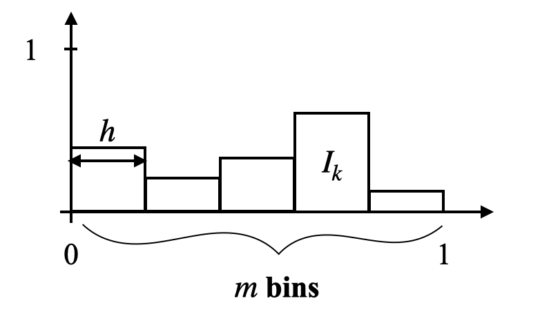
We introduce the hyperparameter \(h \in (0, 1]\), originally noted as \(e\) and called probability sampling step in (Verger et al., 2023), that we rename bandwidth here. Its name, role, and purpose will be further detailed in Section 4, but, as a first intuition, it represents the resolution with which we compute MADD in order to measure fairness with this metric optimally. The bandwidth \(h\) is directly linked to an equivalent parameter, \(m \in \mathbb {N}^{*}\), with \(m\) being equal to \(\lfloor 1/h \rfloor \). Thus, \(m\) is the number of subintervals of the unit interval \(I = [0, 1]\) that the value of \(h\) will determine. Let us see in Figure 1 an illustration of these parameters. In the figure, we can see that \(h\) corresponds to the width of the bins of a histogram (further studied in Section 4) while \(m\) corresponds to its total number of bins. For instance, if \(h=0.022\), then \(m=\lfloor 1/0.022 \rfloor =45\), meaning that there are 45 subintervals of the same width \(0.02\overline {2}\) (or 1/45) in \(I\): \([0, 1/45)\), \([ 1/45, 2/45)\), \(\ldots \), \([43/45, 44/45)\), \([44/45, 1]\). We finally introduce a last notation which is \(I_k\), representing the subinterval indexed by \(k\) where \(I_k = [(k-1) / m, k / m)\) for \(k \in [1, 2, ..., m - 1]\), and \(I_m = [(m-1) / m, 1]\) for \(k=m\). Following up on the above example, \(I_{44} = [43/45, 44/45)\).
3.2. Approach of MADD
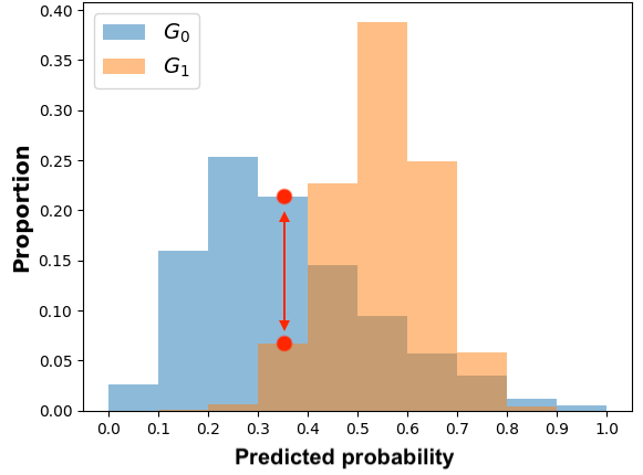
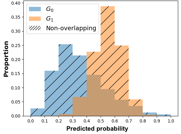
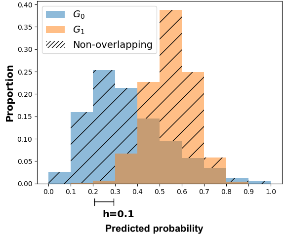
The general idea of MADD consists in comparing how a classifier \(\mathcal {C}\) distributes its predicted probabilities depending on the group the students belong to (\(G_0\) or \(G_1\)). Let us consider a toy example with the distributions displayed in Figure 1a and where \(h=0.1\) so \(m=10\). Thus, to measure how different these distributions are, our goal is to measure the absolute distance between the proportions (or percentages \(\in [0, 1]\)) of students receiving the same probabilities, according to their group membership. For each bin of the two histograms, a single distance corresponds to the red arrow in Figure 1a, and the total distance is consequently the sum of all these single absolute distances. It visually corresponds to the non-overlapping part of the two histograms, as shown in Figure 1b. Indeed, in the areas where the two distributions do not intersect, the model does not distribute its predicted probabilities the same according to the group membership. This is precisely what we intend to measure with MADD.
3.3. Definition of MADD
As previously mentioned in Section 3.2, Model Absolute Density Distance (MADD) is a measure of the absolute distance between the proportions of students of \(G_0\) and \(G_1\) receiving the same predicted probabilities. To define MADD, we first need to introduce two unidimensional vectors, \(D_{G_0}\) and \(D_{G_1}\), that correspond to the two histograms of the respective groups \(G_0\) and \(G_1\), exemplified in Figure 1a. Thus, we denote \(D_{G_0} = (d_{G_0,k})_{1\leqslant k \leqslant m}\) and \(D_{G_1} = (d_{G_1,k})_{1\leqslant k \leqslant m}\), where each \(d_{G_0,k}\) and \(d_{G_1,k}\) is defined such that:
\begin {equation} d_{G_0,k}= \frac {1}{n_0} \sum _{i \in G_0} \mathds {1}_{I_k}(\hat {p}_{i}),\quad d_{G_1,k}= \frac {1}{n_1} \sum _{i \in G_1} \mathds {1}_{I_k}(\hat {p}_{i}) \label {d-k-def} \end {equation}
with \(\mathds {1}\) the indicator function (and \(m\), \(n_0\), and \(n_1\) introduced in Section 3.1). The value of \(\mathds {1}_{I_k}(\hat {p}_{i})\) equals to 1 if \(\hat {p}_{i}\) belongs to the interval \(I_k\) and 0 otherwise:
\begin {equation} \mathds {1}_{I_k}(\hat {p}_{i}) = \left \{ \begin {array}{ll} 1 & \mbox {if } \hat {p}_{i} \in I_k \\ 0 & \mbox {if } \hat {p}_{i} \notin I_k \end {array} \right . \label {indicatorUNDERSCOREfunctionUNDERSCOREeq} \end {equation}
Thus, \(d_{G_0,k}\) (resp. \(d_{G_1,k}\)) contains the proportion of students of \(G_0\) (resp. \(G_1\)) for whom the model \(\mathcal {C}\) gave a predicted probability \(\hat {p}_i\) that fell into \(I_k\). We can now define MADD as follows:
\begin {equation} \label {MADDeq} \text {MADD}(D_{G_0}, D_{G_1}) = \sum _{k=1}^m | d_{G_0,k} - d_{G_1,k} | \end {equation}
The MADD metric satisfies the necessary properties of a metric: reflexivity, non-negativity, commutativity, and triangle inequality (Cha and Srihari, 2002) (see proofs in Appendix of Verger et al. (2023)’s paper). Moreover, a property of MADD is that it is bounded:
\begin {equation} \hspace {0.2cm} 0 \leqslant \text {MADD}(D_{G_0}, D_{G_1}) \leqslant 2 \label {MADDeq-boundaries} \end {equation}
The closer MADD is to 0, the fairer the outcomes of the model are regarding the two groups. Indeed, if the model produces the same probability outcomes for both groups, then \(D_{G_0} = D_{G_1}\) and \(\text {MADD}(D_{G_0}, D_{G_0}) = 0\). Conversely, in the most unfair case, where the model produces totally distinct probability outcomes for both groups, MADD is equal to 2 because we sum all the proportions of both groups whose respective total is 1. An example of such a situation could be when on the one hand, \(\exists k_{0}, d_{G_0,k_{0}} = 1\) and \(\forall k \in [1,m], k \neq k_{0}, d_{G_0,k} = 0\), and on the other hand, \(\exists k_{1} \neq k_{0}, d_{G_1,k_{1}} = 1\) and \(\forall k \in [1,m], k \neq k_{1}, d_{G_1,k} = 0\). In that case, Equation \eqref{MADDeq} simply becomes:
\begin {equation} \text {MADD}(D_{G_0}, D_{G_1}) = | d_{G_0,k_{0}} - 0| + | d_{G_1,k_{1}} - 0| = 1 + 1 = 2 \end {equation}
Also, in Equation \eqref{MADDeq}, we can see that the numerical value of MADD depends on its bandwidth parameter through the value of \(m\) in the sum (see Figure 5 for a visual example). Indeed, since \(m\) is also the number of bins of the histograms, it will affect the \(\hat {p}_i\) that would fall into the \(I_k\) and thus the values of \(d_{G_0,k}\) and \(d_{G_1,k}\). Furthermore, the bandwidth \(h\) allows us to make the two histograms \(D_{G_0}\) and \(D_{G_1}\) comparable for the MADD calculation. Indeed, let us say that the model \(\mathcal {C}\) outputs probabilities in the range of \([0.0, 1.0]\) for one group and of \([0.2, 0.9]\) for the other, such as illustrated in Figure 2. If \(h\) did not allow the discretization of the unit interval \(I=[0, 1]\) to have common bins for both histograms, then the comparison of \(D_{G_0}\) and \(D_{G_1}\) would have been biased and the MADD results would have been wrong estimations of the distance between these two. In Section 4 further on, we will address the selection of this bandwidth parameter \(h\) that allows MADD to best estimate this distance between the two distributions and thus best estimate (un)fairness with this metric.
It is worth emphasizing again, as explained in Section 2.1, that MADD is an independence metric, made for cases where we do not trust the objectivity of the target variable due to complex hidden historical biases. Therefore, a MADD value of 0 only means a fair output according to this definition of fairness. When it is acceptable that two groups have different histograms, e.g., representing a known historical advantage and disadvantage between two groups, this type of fairness should be measured by a separation metric.
3.4. Implementation of MADD
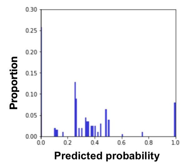
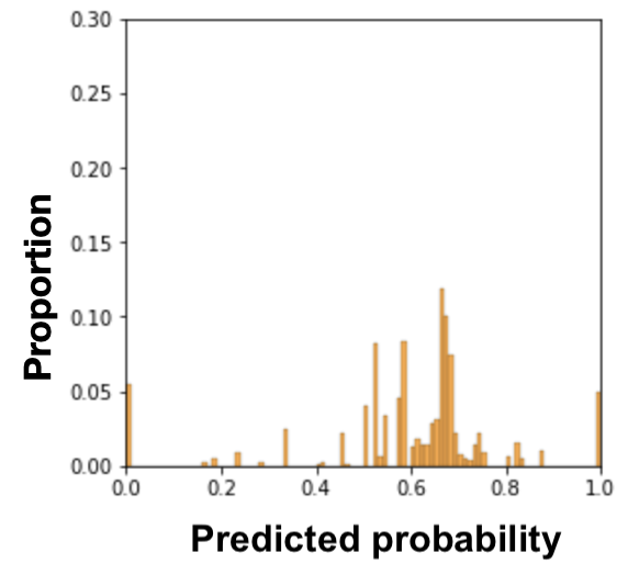
Now, in Figure 3, we show how to compute MADD within a standard ML pipeline. The computation of MADD is performed after the model \(\mathcal {C}\) has been trained, as shown in the dotted box. Hence, it does not affect the data or the model itself. More specifically, MADD is computed on the set of probabilities \(\hat {P}\) outputted by the model. The first step consists in splitting the probabilities pertaining to each group to get \(\hat {P}_{G_0}\) and \(\hat {P}_{G_1}\). An example of this step is provided in Figure 4 with a sample tabular view. Next, the \(D_{G_0}\) and \(D_{G_1}\) vectors are derived from \(\hat {P}_{G_0}\) and \(\hat {P}_{G_1}\) according to the \(h\) parameter, enabling to compute MADD (i.e., Equation \eqref{MADDeq}).
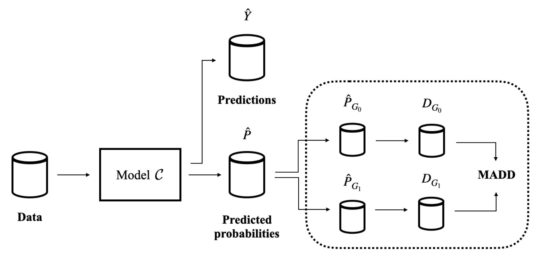

To ease its computation, we created an open-source Python package, maddlib. In particular, it
allows direct computation of MADD when provided with predicted probabilities, i.e., it
performs the split and the computation of \(D_{G_0}\) and \(D_{G_1}\) vectors directly (steps in the dotted box of
Figure 3). It also allows to plot the histograms and distributions for visual analysis. The
instructions for installing and using the package are available at its Python Package Index (PyPI)
link3.
4. Improving MADD computation
In this Section 4, we now focus on the influence of the bandwidth \(h\) on MADD and on how to fine-tune it. In our previous work (Verger et al., 2023), we considered that the choice of \(h\) was to be made by the data analyst based on what seems reasonable in a particular situation. Here, we will first explain how the bandwidth \(h\) intervenes in the MADD calculation (Section 4.1), then we will demonstrate why some optimal bandwidth values always exist (Section 4.2), and we will show how to select them. More precisely, we will provide an automated search algorithm to find this range of optimal bandwidth values (Section 4.3), and we will illustrate our findings on simulated data (Section 4.4) to confirm the validity of our approach, before applying it on real data in the next Section 5.
4.1. Influence of the bandwidth
At the end of Section 3.3, we saw that the bandwidth \(h\) influences the numerical value of MADD. Let us consider the example in Figure 5. When we have a few bins, such as when \(h=0.1\) (left-hand figure), all the probabilities fall into only a few (i.e., \(m=10\)) different intervals \(I_k\), which consequently see their proportions of corresponding \(\hat {p}_i\) increasing. On the other hand, when we increase the number of bins, for example by choosing a lower value of \(h\) such as \(h=0.05\) (right-hand figure), we increase the number of possible intervals (i.e., \(m=20\)) so that the probabilities are distributed into many more different intervals (leading to a visual spread out such as in Figure 4b). Therefore, the value of \(h\) affects the number of bins and thus the values of \(d_{G_0, k}\) and \(d_{G_1, k}\). This, in turn, can influence the numerical value of MADD, e.g., with a MADD of 1.18 for \(h=0.1\) and of 1.19 for \(h=0.05\) in the example of Figure 5.

In the next section, we will show that there exists a range of \(h\) values for which MADD best estimates the distance between the two distributions. Hence, we also call the \(h\) values of this range as optimal \(h\) values or optimal bandwidths. That is why we renamed this parameter as bandwidth (compared to probability sampling step noted \(e\) in (Verger et al., 2023)), as it refers to the range of \(h\) values for which the metric optimally measures (un)fairness.
4.2. Existence of optimal bandwidths
In this Section 4.2, we theoretically (and later experimentally) demonstrate that several optimal \(h\)
values always exist, ensuring that MADD is an optimal measure of (un)fairness, i.e., that it best
estimates the distance between the two distributions. We do so by first showing a property regarding \(D_{G_0}\)
and \(D_{G_1}\) (part 4.2.1), which then leads to demonstrating a theorem about MADD (part 4.2.2). More
specifically, we refine the definition of MADD using a well-established statistical tool, namely
histogram estimators. This enables us to borrow statistical properties from histogram estimators to
determine the optimal \(h\) values (part 4.2.3). In addition to the theoretical proofs, we will provide an
algorithm meant to infer the optimal \(h\) values in practice (next Section 4.3), which is implemented in the
maddlib package3.
4.2.1. Property on \(D_{G_0}\) and \(D_{G_1}\)
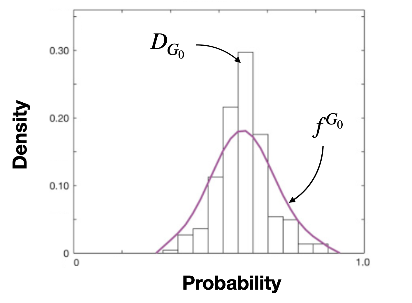
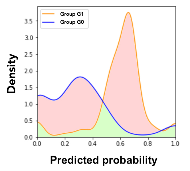
Here, we will see that \(D_{G_0}\) and \(D_{G_1}\) can be considered as probability density estimators. Indeed, the discrete values \(\hat {p}_i\), predicted by a model \(\mathcal {C}\), can be seen as samples of some respective underlying distributions with respect to the group \(G_0\) or \(G_1\). If we note the probability density functions (PDFs) of these underlying distributions as \(f^{G_0}\) and \(f^{G_1}\), therefore we can consider \(D_{G_0}\) and \(D_{G_1}\) as probability density estimators by histograms of \(f^{G_0}\) and \(f^{G_1}\) (Devroye and Gyorfi, 1985). An example is shown in Figure 6.
More precisely, the way we defined \(d_{G_0,k}\) and \(d_{G_1,k}\) in Equation \eqref{d-k-def} corresponds to the definition of a histogram estimator (Devroye and Gyorfi, 1985):
Definition 1. Assume \(f\) is the probability density function of a real distribution, \(\{q_i\}_{1 \leqslant i \leqslant n}\) are the samples of that distribution, and \(\mathds {1}\) the indicator function already defined in Section 3.3. The histogram function of the samples, also called the histogram estimator of \(f\) on \(I = [0,1]\), is: \begin {equation} \widehat {f}_h(x)= \frac {1}{h} \sum _{k=1}^m \left ( \frac {1}{n} \sum _{i=1}^{n} \mathds {1}_{I_k}(q_i) \right ) \mathds {1}_{I_k}(x). \end {equation}
It means that for a given \(h\), we discretize \(I\) in \(m = \lfloor 1/h \rfloor \) intervals \(I_k\) (external sum), and we see for each sample \(q_i\), how many other samples fall into each \(I_k\) (internal sum). Thus, for a \(x \in [0, 1]\), we count the number of \(q_i\) present in the same interval in which \(x\) falls and we divide this number by \(h\) to obtain a proportion. In the end, \(\widehat {f}_h(x)\) simply returns the proportion associated to the interval in which \(x\) falls, given a fixed bandwidth \(h\).
In the case of MADD, the \(\hat {p}_i\) in Equation \eqref{d-k-def} represent the samples \(q_i\) of the respective probability density functions \(f^{G_0}\) and \(f^{G_1}\), and \(d_{G_0,k}\) and \(d_{G_1,k}\) are the respective values of \(\widehat {f}_h(x)\) for the group \(G_0\) and \(G_1\). This property of \(D_{G_0}\) and \(D_{G_1}\) as probability density estimators leads us to a new theorem about MADD (see Theorem 1).
4.2.2. Theorem on MADD
Now, we will see that MADD is in fact a histogram-based estimator of the distance between two distributions on \(L_1[0,1]\) space. Let note \(\widehat {f}^{G_0}_h\), with \(G_0\) superscript, the histogram function of \(f^{G_0}\) (idem with the group \(G_1\)) for a given \(h\). From the previous part, we can interchangeably note \(D_{G_0}\) and \(D_{G_1}\) with \(\widehat {f}^{G_0}_h\) and \(\widehat {f}^{G_1}_h\), which are the histogram functions of \(f^{G_0}\) and \(f^{G_1}\) respectively (that can again be illustrated in Figure 6). Thus, we can formalize MADD as follows (see proof in Appendix 10.1):
Theorem 1___________
\begin {equation} \text {MADD}\left (D_{G_0}, D_{G_1}\right ) = \left \| \widehat {f}^{G_0}_h - \widehat {f}^{G_1}_h \right \|_{L_1[0,1]} \end {equation}
____
Indeed, MADD in its original definition (Equation \eqref{MADDeq}) tries to estimate the distance on \(L_1[0,1]\) space between two distributions, \(f^{G_0}\) and \(f^{G_1}\), thanks to their histogram estimators \(D_{G_0}\) and \(D_{G_1}\). The distance on \(L_1[0,1]\) space is defined as follows (Devroye and Gyorfi, 1985):
Definition 2. Assume \(\widehat {f}^{G_0}_h\) and \(\widehat {f}^{G_1}_h\) are integrable functions on \([0,1]\). The distance between \(\widehat {f}^{G_0}_h\) and \(\widehat {f}^{G_1}_h\) on the space \(L_1[0,1]\) is thus defined as the integral of the absolute value of their difference on \([0,1]\), i.e.: \begin {equation} \left \|\widehat {f}^{G_0}_h - \widehat {f}^{G_1}_h \right \|_{L_1[0,1]} := \int _0^1 \left |\widehat {f}^{G_0}_h - \widehat {f}^{G_1}_h \right | \end {equation}
This measure actually represents, by definition, the area of the disjoint portion of the regions the distributions enclose with the x-axis. Therefore, Theorem 1 can be illustrated in Figure 7 by the red zone that MADD represents, and thus MADD itself can be seen as a histogram-based estimator of the distance between two distributions on \(L_1[0,1]\) space. This result will be crucial to prove the existence of optimal bandwidths in the following part 4.2.3.
4.2.3. Theorem on optimal bandwidths
Since MADD now consists of histogram estimators (part 4.2.1), and thanks to Theorem 1 applicable on \(L_1\) space (part 4.2.2), we can use statistical literature on histogram estimators on \(L_1\) space (Devroye and Gyorfi, 1985) to propose a new theorem on the optimal bandwidths of MADD. Indeed, in the next Theorem 2, we define the \(h\) values with which MADD best estimates (or converges to) the true distance \(\left \| f^{G_0} - f^{G_1} \right \|_{L_1[0,1]}\). We display here a short version of this theorem, but its mathematically rigorous version and its proofs are available in Appendix 10.2.
Theorem 2 (Short version)_________________________
If \(f^{G_0}\) and \(f^{G_1}\) satisfy the commonly required assumptions of smoothness, then
\(\text {MADD}\left (D_{G_0}, D_{G_1}\right )\), whose \(D_{G_0}\) and \(D_{G_1}\) depend on \(h\), converges to \(\left \| f^{G_0} - f^{G_1} \right \|_{L_1[0,1]}\)
with the smallest error (of at most \(O\left (\left ( \frac {\sqrt {n_0} + \sqrt {n_1} }{ \sqrt {n_0 n_1}} \right )^{\frac {2}{3}}\right )\)), when \(h=O\left (\left ( \frac {\sqrt {n_0} + \sqrt {n_1} }{ \sqrt {n_0 n_1}} \right )^{\frac {2}{3}}\right )\).
_________
There are three important points to highlight from this theorem. Let note \(c = \left ( \frac {\sqrt {n_0} + \sqrt {n_1} }{ \sqrt {n_0 n_1}} \right )^{\frac {2}{3}}\). Firstly, when the number of samples or students \(n\) increases, MADD converges to the true distance between the two distributions, \(\left \| f^{G_0} - f^{G_1} \right \|_{L_1[0,1]}\). It is exemplified later on in Figure 10b. Secondly, when MADD precisely converges to the true distance, the errors between MADD and the true distance are at most \(O(c)\), i.e., in order of \(c\). For simplification, the notation \(O(c)\) means that, if the errors are \(O(c)\), then they are inferior or equal to \(c\) multiplied by a constant \(k > 0\). Another way to apprehend the notation \(O\) is that the errors are asymptotically smaller or equal to \(c \times k\). Thirdly, and most importantly for the search of optimal bandwidths, the smallest error is reached when \(h\) is \(O(c)\). Again, it means that the optimal \(h\) this time should be inferior or equal to \(c \times k\). We will note \(h_{sup} = c \times 1 = c\) in the rest of the paper. In the end, we now know that MADD converges to a specific value, which is the best estimate of the true distance, and leading to a range of optimal \(h\) values around \(h_{sup}\).
If we knew the theoretical \(f^{G_0}\) and \(f^{G_1}\), we could find a single precise optimal \(h\) for which MADD is the very best estimate of \(\left \| f^{G_0} - f^{G_1} \right \|\). In practice, since we only have access to their histogram estimations \(D_{G_0}\) and \(D_{G_1}\) (or \(\widehat {f}^{G_0}_h\) and \(\widehat {f}^{G_1}_h\)), we can only identify the range of optimal \(h\) values. Consequently, in the following section, we elaborate on a search strategy to approximate this range of \(h\) values for which MADD optimally estimates (un)fairness.
4.3. Optimal Bandwidth Interval Search Algorithm
Now that we know that optimal bandwidths always exist, the question is: how can we find them in practice? To this end, we developed Algorithm 1, presented in the next pages, to infer these \(h\) automatically. We will first discuss the approach taken by the algorithm in part 4.3.1, followed by a detailed description of how the algorithm works in part 4.3.2.
4.3.1. Approach
As said in the previous part 4.2.3, Theorem 2 ensures that MADD will converge to the true distance \(\left \| f^{G_0} - f^{G_1} \right \|_{L_1[0,1]}\) for a range of \(h\) that we will call optimal bandwidth interval in the following. Although we cannot know the single precise optimal \(h\) in practice, we can still identify an optimal bandwidth interval where MADD has converged and is considered “stable”. In this context, “stable” implies that the MADD values remain consistent, i.e., within a range that we will assess with the smallest standard deviation possible.
To find this optimal bandwidth interval, since \(h \in (0, 1]\) (Section 3.1), we first compute MADD for a large given number of \(h\) within the search space \((0,1]\) (e.g., we chose \(1,000\) distinct \(h\) values in Section 4.4, and the more the better depending on computation time). Then, we explore all possible eligible intervals of \(h\), whose conditions are below, within this search space, and we compute the standard deviation of the MADD values within each eligible interval to find the one with the smallest standard deviation. Nonetheless, as \(h_{sup}\) is already a compromise between the number of students \(n_0\) and \(n_1\) (part 4.2.3), it is most likely that \(h\) will be smaller than \(h_{sup}\) for better precision, which means that the experimental optimal \(h\) will be expected to lie before \(h_{sup}\) in the search space.
To define eligible intervals, we set two conditions. Firstly, each eligible interval should include at
least 50 MADD values minimum to ensure that the standard deviation is meaningful (\(nbPointsMin\) in Algorithm 1).
This condition comes from the fact that distinct MADD values are associated to \(h\) values that are not
linearly spaced, as explained in the next paragraph. Secondly, the width of the eligible intervals is set to
at least \(h_{sup} \times 0.45\) (\(percent\) in Algorithm 1) to ensure that MADD appears stable within a significantly large range, which
is unlikely due to chance. It has to be noted that the values of these two conditions, which we deem
reasonable based on our experience, are nonetheless arbitrary and can be fine-tuned in the maddlib
package3.
As a final remark, Algorithm 1 should thus be provided with a list of \(h\) values representing the search
space within which to find the stable interval, i.e., the optimal bandwidth interval. More precisely, to
compute this list, it is important to note that it is not necessary to consider every possible discrete \(h\)
within \((0, 1]\). Indeed, an infinity of particular \(h\) would yield the same number of bins \(m\), which does not affect
the resulting MADD value. For instance, both \(h = 0.7\) and \(h = 0.6\) lead to the same \(m = \lfloor 1/h \rfloor = 1\) bin, as well as \(h = 0.71\), \(h = 0.711\), \(h = 0.7111\), and so on.
Therefore, we propose to compute the relevant values of \(h\) directly from a list of distinct \(m\) values,
handled in the maddlib package (see the getting-started tutorials3). For instance, let us
assume that we want to find the optimal bandwidth interval considering a search space
with only 5 \(h\) values, as a toy example. We first compute \(m = [1, 2, 3, 4, 5[\) that we turn by definition (\(\lfloor 1/h \rfloor \)) into \(h = [1, 0.50, 0.3\overline {3}, 0.25, 0.2[\),
finally reversed to become the search space \(h = ]0.2, 0.25, 0.3\overline {3}, 0.50, 1]\). Repeating this process with a large number
of \(m\) or \(h\), e.g., 500, the larger the \(m\), the smaller the \(h\). Thus, in the resulting search space, the
small \(h\) values are finer-grained (e.g., \(\lfloor 1/498 \rfloor \) vs. \(\lfloor 1/499 \rfloor \)) than the higher ones (e.g., \(\lfloor 1/2 \rfloor \) vs. \(\lfloor 1/3 \rfloor \)). That is why
MADD will look like a step function with respect to \(h\) (see Figures 9 and 10), since the
MADD value changes only when the value of \(h\) is derived from a distinct number of bins
\(m\).
4.3.2. Description
We now describe Algorithm 1 that we designed to perform the optimal bandwidth interval search defined above. Firstly, in lines 2-6, we take as inputs the list of \(h\) values to look for the stable interval, then the corresponding MADD values for each \(h\), the number of individuals in both groups \(G_0\) and \(G_1\), \(nbPointsMin\) set to 50 and \(percent\) set to 0.45 by default, as said in the previous part 4.3.1. After that, in lines 12 to 14, we initialize the variables to be updated during the search, and in lines 15 and 16, we compute the \(order\) as defined as \(h_{sup}\) based on Theorem 2, and infer \(intervalLengthMin\) from it.
Secondly, from lines 18 to 37, we start the search by delimiting an eligible interval with its left index \(i\) and its right index \(j\) (there are two “for” loops over \(i\) and \(j\) respectively). In line 21, if its lower bound, derived from the left index \(i\) (\(Lh[i]\) line 19), is already too large, the desired minimal length of the interval cannot be achieved and the loop stops (lines 21-23). Otherwise, between lines 24-28, we build this interval with an initial length \(intervalLengthMin\) (line 24) and we check if there are enough MADD values (\(nbPointsMin\)) into it (lines 25-26). If not, we extend it to reach \(nbPointsMin\) (line 27). Then, the right index \(j\) moves forward from the end of the considered interval to the end of the list of all possible \(h\) (line 30; \(Lmadd\) contains the same number of elements as \(Lh\)). Thus, all eligible intervals, between \(i\) and \(j\) indexes, are considered, and we compute the standard deviation of MADD values for each of them (lines 30-36). If an interval comes up with a standard deviation smaller than the previously saved one, then we update \(stdMin\) and the \(indexes\) with the information of the newly selected interval. We repeat this process moving forward \(i\) index, too (two “for” loops). This enables to find the most stable interval as defined in the previous part, i.e., with the smallest standard deviation.
At the end of Algorithm 1, we output, as presented in lines 8 to 10, the information about the optimal interval where the stable value of MADD is the best estimate of (un)fairness between the groups \(G_0\) and \(G_1\). In the next Section 4.4, we illustrate the search of optimal bandwidths with simulated data.
4.4. Application with Simulated Data
Here, to showcase the effectiveness of our automated search algorithm and how the theoretical findings can be illustrated (e.g., convergence, order of \(h\)), we run an experiment via simulated data. Here, simulated data allows us to know the expected results so that we can compare these with the results we obtain with our approach, which is not the case in practice. Experiments with real-world data are rather conducted in Section 5 to replicate our previous work (Verger et al., 2023) with optimal bandwidths. After introducing the simulated distributions and the bandwidths we will work with (parts 4.4.1 and 4.4.2), we empirically observe the convergence of MADD in the optimal bandwidth interval (part 4.4.3), and how our automated search algorithm is able to determine the stable MADD value that is the best estimate of the distance between the two distributions (part 4.4.4).
4.4.1. Simulated data
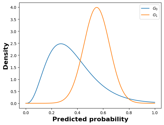
We simulate \((\hat {p}_i)_{i \in G_0}\) and \((\hat {p}_i)_{i \in G_1}\) as if they have been obtained from the output of a classifier. Let \((\hat {p}_i)_{i \in G_0}\) and \((\hat {p}_i)_{i \in G_1}\) be samples of some respective PDFs \(f^{G_0}\) and \(f^{G_1}\). We choose two arbitrary PDFs \(f^{G_0}\) and \(f^{G_1}\) so as to simulate a scenario where the model tends to give higher probabilities to the group \(G_1\) over the group \(G_0\). As displayed in Figure 7a, we define them as part of the gamma distribution \(\Gamma (4,1)\) and the normal distribution \(\mathcal {N}(0.55,1)\) respectively, properly scaled along the x-axis thanks to coefficients \(10\) and \(11\), and normalized within the interval \([0, 1]\):
\begin {equation} \begin {alignedat}{2} f^{G_0}(x) &:= \frac {1}{C_0} f_{\Gamma (4,1)} (11x) \mathds {1}_{[0,1]}(x) &\quad &C_0:=\int _0^1 f_{\Gamma (4,1)} (11x) dx \\ f^{G_1}(x) &:= \frac {1}{C_1} f_{\mathcal {N}(0.55,1)} (10x) \mathds {1}_{[0,1]}(x) &\quad &C_1:=\int _0^1 f_{\mathcal {N}(0.55,1)} (10x) dx \end {alignedat} \end {equation}
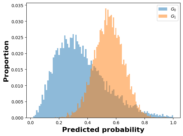
Based on the above PDFs, we generate \(10,000\) samples of \({(\hat {p}_i)}_{i \in G_0}\) and \(10,000\) samples of \({(\hat {p}_i)}_{i \in G_1}\), whose vectors \(D_{G_0}\) and \(D_{G_1}\) can be illustrated in Figure 7b.
4.4.2. Bandwidth search space
We compute \(1,000\) values of \(h\) into \((0, 1]\), on the one hand, to examine a large number of them inside the search space to find the optimal ones, and on the other hand, to show that the optimal bandwidth interval can indeed be found before \(h_{sup}\). As highlighted at the end of part 4.3.1, they are not regularly spaced since different \(h\) values could lead to the same number of bins \(m\), and thus create some redundancy in the results. Therefore, we generate \(1,000\) values of \(m\) linearly spaced by 1, and for each of them, we calculate the corresponding \(h\). We remind that, as a consequence, we have many more \(h\) concentrated towards the small values (when \(m\) is higher), which we can see in Figures 9 and 10.
4.4.3. Convergence of MADD and optimal bandwidth interval
Now that we have defined the distributions and the bandwidths of study, our goal is twofold: to observe an effective convergence of MADD (to a specific value), and to verify that the optimal bandwidth interval is indeed situated before \(h_{sup}\), given Theorem 2.
To do so, we analyze the difference between MADD, i.e. \(|| \widehat {f}^{G_0}_h - \widehat {f}^{G_1}_h ||_{L_1[0,1]}\) (as defined in Theorem 1), and the true distance \(|| f^{G_0} - f^{G_1} ||_{L_1[0,1]}\) that MADD is meant to estimate. While we cannot access the latter in practice, here, with simulated data, we can check if MADD indeed converges to the true distance, i.e., if we are able to observe a stable zone of errors between both as well as if this zone is located before \(h_{sup}\).
Let \( A = { \left | \text {MADD}\left (D_{G_0}, D_{G_1}\right ) - || f^{G_0} - f^{G_1} ||_{L_1[0,1]} \right | }\) be the error between MADD and the true distance. We want to observe how \(A\) varies across all \(h\) values to see when \(A\) is the smallest or even null, meaning that MADD best estimates the true distance.
In Figure 8a, we can first see that when \(h\) becomes greater than about \(0.1\), \(A\) increases rapidly. It means that a too large \(h\) leads to inaccurate MADD results. Therefore, it is not advisable to have less than \(m=10\) bins.
If we zoom on the smallest \(h\) values in Figure 8b, we can observe an interval of bandwidths where \(A\) is null, meaning that MADD provides optimal results. This interval, between the green vertical dotted lines, expectedly falls before \(h_{sup}\) which is equal to \(h_{sup} = \left (\frac {100+100}{10000}\right )^{\frac {2}{3}} \approx 0.074\) and illustrated by a red vertical dotted line.


4.4.4. Automated search of optimal bandwidths with our proposed algorithm
Our goal now is to check if our automated search algorithm is able to determine where is the optimal bandwidth interval as well as the stable MADD value (the best estimate of the distance between the two distributions). To do so, we test Algorithm 1 to identify the above-mentioned interval in part 4.4.3, without knowing the exact distance between the distributions via \(A\). We look directly at the MADD results instead of \(A\) as we would do in practice.
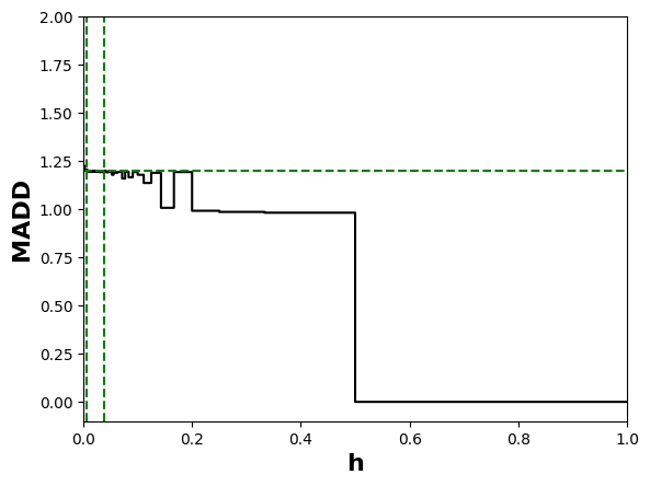
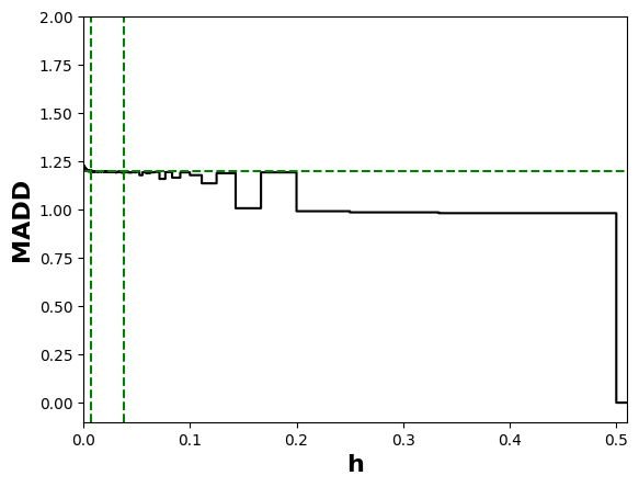
Thus, we plot MADD according to the \(h\) values in Figure 10. Then, we use our Algorithm 1 to find the optimal bandwidth interval. We can observe in this figure that MADD converges to a specific value as expected. Our automated search algorithm successfully identified the optimal interval, enclosed between the green vertical dotted lines. In this interval, the average MADD value is \(1.19\), illustrated by a green horizontal dotted line. This value is consequently the most accurate MADD measurement for this simulated scenario, with the distributions displayed in Figure 8.
More precisely, this optimal interval, found by the algorithm, is \(h \in [0.007, 0.040]\) (included before \(h_{sup} \approx 0.074\)). Therefore, a practical bandwidth \(h\) chosen from this interval will provide a stable and accurate MADD value, closest or even equal to the true distance \(\left \| f^{G_0} - f^{G_1} \right \|_{L_1[0,1]}\). To transition to real data, we will also study the influence of the number of samples or students in a dataset in the next Section 4.5.
4.5. Influence of the number of samples
Additionally to the bandwidth, we will briefly study the influence of the number of samples on the MADD computation. Not only are the bandwidths important to an accurate measurement, but the number of samples plays a role, too. Indeed, as we saw in Theorem 2, \(h_{sup}\) depends on \(n_0\) and \(n_1\).
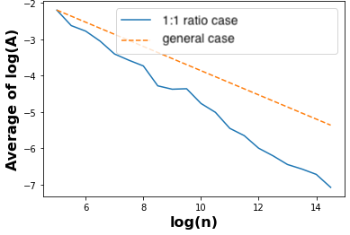
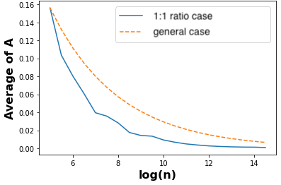
Our objective here is to compute the error \(A = \left | \text {MADD}\left (D_{G_0}, D_{G_1}\right ) - || f^{G_0} - f^{G_1} |_{L_1[0,1]} \right |\) according to various sample sizes. We remind that \(n\) is the total number of samples, where \(n = n_0 + n_1\) (Section 3.1). We experiment with various \(n\) values taken from the following set: \(\{ \lfloor \exp (5) \rfloor , \lfloor \exp (5.5) \rfloor , \cdots , \lfloor \exp (14.5) \rfloor \}\), as shown on the x-axis in Figure 11. We repeat each calculation of \(A\) for each \(n\) 50 times to account for the variability resulting from the sampling of the probabilities that represent the two distributions. In the subsequent paragraphs, we will analyze the case where \(n_0\) and \(n_1\) are balanced as well as the general case where they are unbalanced thanks to theoretical considerations, using optimal \(h\) values for both scenarios.
Firstly, we set a 1:1 ratio for \(n_0\) and \(n_1\) so that \(n_0 = \lfloor n/2 \rfloor \). In Figure 11, the blue solid line represents the error in this scenario. In Figure 10a, we observe a linear decrease in logarithmic error as the logarithmic sample size \(n\) increases. This implies that the accuracy of MADD improves with an increase in \(n\). We plot the actual errors \(A\) without the logarithmic scale in Figure 10b to provide a more intuitive understanding of this trend, the blue solid line converging to a null error. We notice that for a small dataset, when \(n=\lfloor \exp {(6)} \rfloor = 403\), the error is only \(0.08\) (\(4\%\) error). For a small or medium-sized dataset, when \(n=\lfloor \exp {(8)} \rfloor = 2981\), the error is \(0.028\) (\(1\)% error). For larger datasets, the error is nearly zero, indicating that MADD is the most accurate estimate of (un)fairness.
Secondly, for other ratios of \(n_0\) and \(n_1\), i.e., for the most general case, we will take the logarithm of \(\left ( \frac {\sqrt {n_0} + \sqrt {n_1} }{ \sqrt {n_0 n_1}} \right )^{\frac {2}{3}}\) to determine its relationship with \(n\) by linearization (transforming power into multiplicative factor). To do so, we introduce two ratios \(0 < \alpha = n_0/n < 1\) and \(\beta = 1 - \alpha \), and we obtain the following, by substituting \(n_0\) and \(n_1\) by \(\alpha \) and \(\beta \) (see proof in Appendix 10.3):
\begin {equation} \label {eq:logUNDERSCOREcvUNDERSCOREspeed} \log \left ( \left ( \frac {\sqrt {n_0} + \sqrt {n_1} }{ \sqrt {n_0 n_1}} \right )^{\frac {2}{3}} \right ) = -\frac {1}{3} \left ( \frac {\alpha \beta }{1+2\sqrt {\alpha \beta }} \right ) -\frac {1}{3} \log (n) \end {equation}
According to this equation, we see that \(\log \left ( \left ( \frac {\sqrt {n_0} + \sqrt {n_1} }{ \sqrt {n_0 n_1}} \right )^{\frac {2}{3}} \right )\) has a linear relationship with \(\log (n)\) (with a coefficient of \(-1/3\) and an intercept of \(-\frac {1}{3} \left ( \frac {\alpha \beta }{1+2\sqrt {\alpha \beta }} \right )\)). This means that, for any different ratios of \(n_0\) and \(n_1\), we will also observe a linear decrease of the logarithmic errors when \(n\) increases, as the 1:1 ratio scenario. Indeed, we observe the above linear relationship in both Figures 10a and 10b thanks to orange dotted lines, following the trend of the 1:1 scenario.
Moreover, with the two scenarios displayed in the same figure, we can see that when \(n_0\) and \(n_1\) are balanced (blue solid line), MADD converges (to the true distance \(\|f^{G_0} - f^{G_1}\|_{L_1}\)) with even lower errors than the general case in orange dotted lines (the blue line has a better coefficient of \(-0.51 < -1/3\)).
As a summary, MADD is friendly to large but also small datasets, and for different ratios of \(n_0\) and \(n_1\), all the more when the number of samples \(n\) increases.
5. Replication of (Verger et al., 2023) experiments
We now aim to replicate the experiments reported in our previous work, but using the bandwidth search algorithm we proposed above (Algorithm 1) to find the optimal \(h\) values for computing MADD. To do so, we leverage the same dataset that we used in (Verger et al., 2023), namely the Open University Learning Analytics Dataset (OULAD) (Kuzilek et al., 2017). In Section 5.1, we will first provide a high-level description of the experimental setup. Further information about the choices of the data and models can be found in (Verger et al., 2023). Then, in Sections 5.2 and 5.3, we will present the updated results.
5.1. OULAD Dataset and Models
The dataset we used in our study is sourced from The Open University, a distance-learning institution based in the United Kingdom, and concerns student activity and demographics between 2013 and 2014. Notably, the dataset includes information on at least three sensitive features, namely gender, poverty, and disability (see Table 1). Our research aims to evaluate the fairness of classifiers that predict whether a student will pass or fail a course, using this data. As in (Verger et al., 2023), among the seven courses provided in the OULAD dataset, we chose two specific courses, labeled as “BBB” and “FFF”, with a total of \(7,903\) and \(7,758\) enrolled students, respectively.
In particular, the passing rate in these two courses was to some extent correlated with the gender feature. Thus, they were good candidates for examining the impact of gender bias on the predictive models’ fairness. Moreover, the “BBB” course corresponds to a Social Sciences course and the “FFF” course to a STEM (Science, Technology, Engineering, and Mathematics) course, making them relevant candidates for examining the impact of gender bias on the predictive models’ fairness on two different student populations. In addition, both courses presented very high imbalances in terms of disability (respectively \(91.2\)-\(8.8\)% and \(91.7\)-\(8.3\)% for the not disable-disable groups in courses “BBB” and “FFF”) and gender (respectively \(88.4\)-\(11.6\)% and \(17.8\)-\(82.2\)% for female-male groups in courses “BBB” and “FFF”), and still some imbalance for poverty (respectively \(42.3\)-\(57.7\)% and \(46.9\)-\(53.1\)% for less-more deprived groups in courses “BBB” and “FFF”). Based on these preliminary unfairness expectations derived from the skews in the data, it is interesting to analyze whether and how the models will suffer from these biases in both courses. Indeed, by nature, imbalanced data means there is less representation of the minority groups, making it harder to train a ML model from them than from the majority group. It is therefore a plausible initial hypothesis that the models trained here may lead to a higher error rate for the minority groups.
The features we use to predict whether a student will pass or fail a course are displayed in Table 1.
Regarding the three sensitive features considered in this study, it is questionable to use demographic
information during training (Baker et al., 2023), but since we precisely want to
understand how these sensitive features play a role in the models’ outcomes, we kept them. The
sum_click feature was the only one that was not immediately available as is, and we computed it
from inner joins and aggregation on the original data. Then, we learn out-of-the-box classifiers on this
data, using a \(70\)-\(30\)% split ratio between the training and the test sets. We use the exact same classifiers as in
(Verger et al., 2023) for the sake of comparison, namely a logistic regression classifier
(LR), a k-nearest neighbors classifier (KN), a decision tree classifier (DT), and a naive Bayes classifier
(NB).
The accuracy of the trained classifiers was above a majority-class baseline (\(70\)%), and up to \(93\)% for DT, except for the NB (\(62\)%) which instead presented interesting behaviors in the previous analyses and was deemed worth keeping it. It is important to note that our experiments focused on analyzing fairness in widely used models rather than solely achieving optimal predictive performance, which is typically the goal of most ML studies. Thus, in a practical application, the initial aim would be to find models with acceptable predictive performance and subsequently use the MADD method to select the fairest options from that set.
To compute MADD, we use the bandwidth search algorithm we proposed (Algorithm 1) to find the optimal \(h\) values for each combination of models and demographics in both “BBB” and “FFF” courses, i.e., for every measurement. This approach not only demonstrates the practical application of our search algorithm in real-world educational data but also enables us to compare MADD results when using an optimal bandwidth vs. a predefined one, as previously done in (Verger et al., 2023). We remind that, in our previous work, the bandwidth parameter was arbitrarily set to \(0.01\), corresponding to a variation of the probability of success or failure of \(1\)%.
| Name | Feature type | Description |
|---|---|---|
gender\(^*\) | binary | students’ gender |
age | ordinal | the interval of students’ age |
disability\(^*\) | binary | indicates whether students have declared a disability |
highest_education | ordinal | the highest student education level on entry to the course |
poverty\(^*\)4 | ordinal | specifies the Index of Multiple Deprivation (Kuzilek et al., 2017) band of the place where students lived during the course |
num_of_prev_attempts | numerical | the number of times students have attempted the course |
studied_credits | numerical | the total number of credits for the course students are currently studying |
sum_click | numerical | the total number of times students interacted with the material of the course |
5.2. Results for Course “BBB"
We present both the MADD results previously obtained from (Verger et al., 2023), in Table 2, and the updated MADD results computed with optimal bandwidths, in Table 3. We highlight in bold, in the latter table, the MADD results that do not change after the optimal computation, and we add for each measurement its corresponding optimal bandwidth interval.
|
Model | Sensitive features | ||||
gender | poverty | disability | Average | ||
|
MADD | LR | 1.72 | 1.85 | 1.57 | 1.71 |
| KN | 1.13 | 1.12 | 0.93 | 1.06 | |
| DT | 0.69 | 0.85 | 0.65 | 0.73 | |
| NB | 0.52 | 0.9 | 1.37 | 0.93 | |
| Average | 1.02 | 1.18 | 1.13 | ||
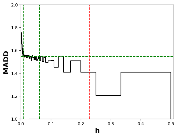
Comparing Tables 2 and 3, we see that 7 of the 12 MADD values are identical, in particular for the KN and DT models. Indeed, these models, by definition of their inner workings, already output only a few discrete values of possible predicted probabilities (see Figures 4 and 5 from (Verger et al., 2023) as examples). In the case of the KN model, it does not inherently provide a continuous probability distribution, as the predicted probability for a class is based only on the proportion of neighbors belonging to that class within the local neighborhood. In the case of the DT model, its predictions are inherently discrete and simply cannot provide a continuous probability distribution. Therefore, their MADD values are extremely stable for any number of bins \(m\) and thus for any \(h\) values, which is shown in Figure 12. As for the 5 other MADD values that are not identical to the previous results, they are on average \(1.3\)% different (\(0.026\) error on average), which is very low. This is due to the fact that even when it was not inside the optimal bandwidth interval, the \(h\) value empirically chosen in that paper was always very close to it.
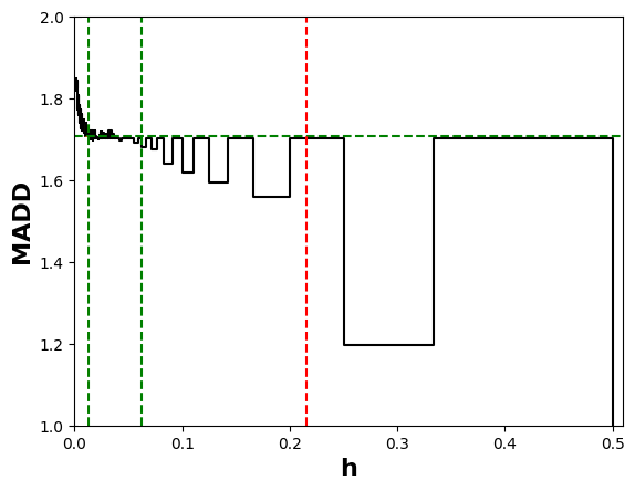
These results show not only that the conclusions from (Verger et al., 2023) still hold, but also that we can now safely exclude that a poor choice of \(h\) might have unfairly and artificially increased the MADD value for one of the tested classifiers. In particular, while we expected that gender and disability would generate more algorithmic unfairness as discussed above (Section 5.1), MADD is actually the worst for poverty on average (\(1.17\), see Table 3). Furthermore, trained on the same data, the models exhibit different levels of algorithmic unfairness (e.g., NB is the most fair for gender whereas DT and KN are the most fair for disability). This does confirm the need to investigate and compare systematically the fairness of different models on a given dataset.
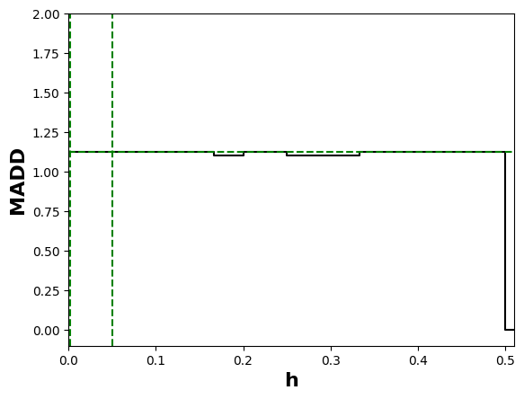
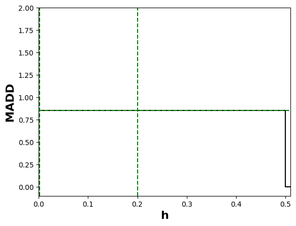
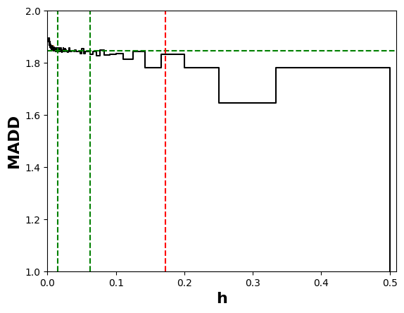
As for the search algorithm, Figure 12 also shows that for classifiers like DT and KN that output a few discrete probabilities (e.g., \(0\), \(0.5\), and \(1\) for DT), it is rather trivial to find an optimal \(h\). Thus, for completeness, we also showcase in Figure 13 the output of Algorithm 1 on the LR classifier that provides more continuous probabilities. Figure 13 shows similar findings than with the simulated data above, confirming that the algorithm can effectively identify the optimal bandwidth intervals with real-world data, too.
5.3. Results for Course “FFF"
For this course, we present the previous results in Table 4 and the current results in Table 5. Again, we highlight in bold, in the latter table, the results that do not change after choosing an \(h\) value within the optimal bandwidth intervals. We see that 6 of the 12 MADD values are identical, again for the KN and DT models for the same reason as previously. For the other 6 values, they are on average \(3.5\)% different (\(0.07\) error on average), which is still quite low and therefore does not jeopardize the conclusions drawn from experiments described in (Verger et al., 2023).
Our algorithm thus obtains successful results also for real-world educational data, where the number of samples in the dataset is limited (\(1,590\) and \(1,422\) in the respective test sets of the courses “BBB” and “FFF”) and the types of distributions scattered compared to simulated data. Now, in the next Section 6, we will demonstrate how MADD can be used not only to measure unfairness, but also to mitigate it through post-processing of the model output while preserving its accuracy as much as possible.
|
Model | Sensitive features | ||||
gender | poverty | disability | Average | ||
|
MADD | LR | 1.18 | 1.06 | 1.12 | 1.12 |
| KN | 1.06 | 0.93 | 0.78 | 0.92 | |
| DT | 0.76 | 0.65 | 0.55 | 0.65 | |
| NB | 0.56 | 0.47 | 0.90 | 0.64 | |
| Average | 0.89 | 0.78 | 0.84 | ||
6. Improving fairness with MADD
In this Section 6, we propose to use the MADD metric to mitigate algorithmic unfairness. To do so, we develop a post-processing method based on MADD, which modifies the initial predicted probabilities of a model to fairer probabilities and thus predictions.
6.1. The MADD Post-Processing Approach
6.1.1. Purpose
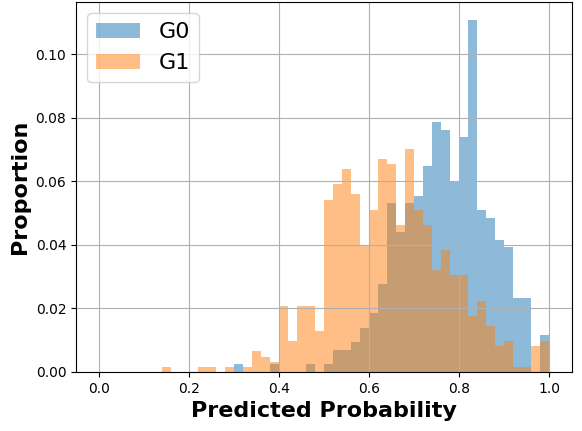
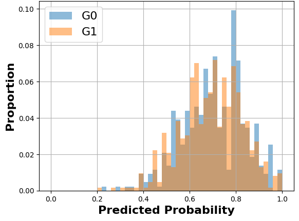
As introduced in Section 3, the closer MADD is to 0, the fairer the outcome of the model is (w.r.t to attribute \(S\)), since the distributions of predicted probabilities are no longer distinguishable regarding the group membership (\(G_0\) or \(G_1\)). Thus, to illustrate how the post-processing with MADD would work, we consider a toy example with a model that tends to give higher predicted probabilities (i.e., probabilities of success predictions) to a group than to the other, as shown in Figure 13a. Therefore, the goal of the MADD post-processing is to reduce the gaps between the distributions of both groups, to obtain a result similar to what we can observe in Figure 13b.
6.1.2. Approach
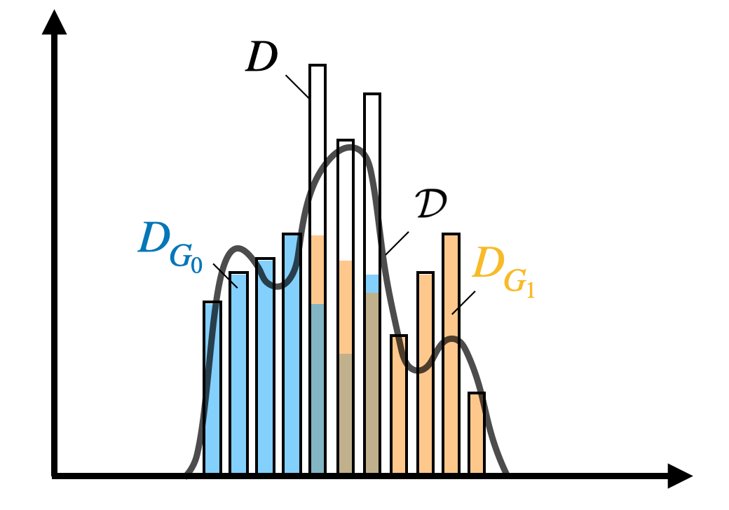
Following up on the previous part, a question can be raised: where should the two distributions coincide? Indeed, should the distribution of \(G_1\) move to the one of \(G_0\), or is there a better location between the two? To solve this issue, let us first note as \(D\) the distribution related to all students, composed of students from both groups \(G_0\) and \(G_1\) (see the black histogram in Figure 14a). In machine learning, the goal for a model is to approximate the “true” relationship (or prediction function \(\mathcal {X} \rightarrow \mathcal {Y}\)) between the attributes \(X\) in input and the target variable \(Y\) in output. As a consequence, we assume that a model that shows satisfying predictive performance outputs a discrete distribution \(D\) which should be really close to \(\mathcal {D}\), its “true” distribution (see the black line in Figure 14a). Therefore, assuming having such a model, our goal is to make the distributions \(D_{G_0}\) and \(D_{G_1}\) coincide at the place of \(D\), which should best approximate \(\mathcal {D}\). Indeed, this allows both to reduce the gaps between the two groups, hence improving fairness and preventing a loss in predictive performance. Therefore, the MADD post-processing is based on the following theoretical considerations.
As seen earlier in part 4.2.1, since \(D\), \(D_{G_0}\) and \(D_{G_1}\) correspond to histograms, they can be mathematically considered as estimators of the PDFs they describe (see Figure 6) (Devroye and Gyorfi, 1985) and noted as \(f\), \(f^{G_0}\) and \(f^{G_1}\) respectively. We thus want \(f^{G_0}\) and \(f^{G_1}\) to move towards the target \(f\), as the intuition was given in the previous paragraph. To define how these functions should get closer, we define the new theoretical PDFs \(\widetilde {f}\), \(\widetilde {f}^{G_0}\) and \(\widetilde {f}^{G_1}\) that will be estimated thanks to the post-processing. Thus, \(f, f^{G_0}\), \(f^{G_1}\), \(\widetilde {f}^{G_0}\), and \(\widetilde {f}^{G_1}\) should be colinear (see Figure 14b for an illustration and see proof in Appendix 10.4). As a consequence, the ratio between \(\widetilde {f}^{G_0}\) and \(f\) and between \(\widetilde {f}^{G_1}\) and \(f\) remains constant (as shown in Figure 14b), which prevents improving fairness more for one group than for the other. By introducing a \(\lambda \) parameter, that we call fairness coefficient of distribution convergence, such that: \begin {align} \widetilde {f}^{G_0} = (1-\lambda ) f^{G_0} + \lambda f \label {eq:2} \\ \widetilde {f}^{G_1} = (1-\lambda ) f^{G_1} + \lambda f \label {eq:3} \end {align}
\(\lambda \) can be seen as a distance ratio (see Figure 14b) so that \(\lambda \in [0, 1]\), with \(\lambda = 0\) when the PDFs of \(G_0\) and \(G_1\) are at their
initial state and \(\lambda = 1\) when they both coincide. \(\lambda \) between 0 and 1 means that the distributions are getting
closer (see discrete examples of distribution convergence in Figure 17, later). The challenge is to find
the highest \(\lambda \) possible that best improves the fairness without affecting the accuracy of the results.
However, in practice, as we do not know the true \(f\), \(f^{G_0}\) and \(f^{G_1}\), we cannot directly compute \(\widetilde {f}\), \(\widetilde {f}^{G_0}\) and \(\widetilde {f}^{G_1}\) as written in
Equations \eqref{eq:2} and \eqref{eq:3} with different values of \(\lambda \). That is why we introduce fip in
the next part.
6.1.3. Implementation
We will generate a mapping function5,
fairness_improved_prediction or in short fip, between the discrete estimates of \(f\), \(f^{G_0}\), \(f^{G_1}\) (i.e. \(D\), \(D_{G_0}\), \(D_{G_1}\))
and the discrete estimates of \(\widetilde {f}\), \(\widetilde {f}^{G_0}\), \(\widetilde {f}^{G_1}\) that we will note as \(\overline {D}\), \(\overline {D}_{G_0}\), \(\overline {D}_{G_1}\). The purpose of fip is more precisely to take as
inputs the \(\hat {p}_i\) available at the output of a trained model and a value of \(\lambda \), and to output the new fairer
predicted probabilities that we note as \(\overline {p}_{i}^{(\lambda )}\) (fip: \((\hat {p}_i\), \(\lambda )\) \(\mapsto \) \(\overline {p}_{i}^{(\lambda )}\)). Consequently, \(\overline {p}_{i}^{(\lambda )}\) will allow to reconstruct the new \(\overline {D}_{G_0}\) and
\(\overline {D}_{G_1}\), as shown in Figure 13b.
fip will be generated as follows. Let us focus on the group \(G_0\) first. As we want the proportions of
students having the same predicted probabilities to be kept even if the predicted probabilities values are
changing with the post-processing, we will seek to make the cumulative density function (CDF) of the
initial \(\hat {p}_i\) of group \(G_0\) being equal to the CDF of the new \(\overline {p}_{i}^{(\lambda )}\) of group \(G_0\). Thus, it comes that (see proof in
Appendix 10.5):
\begin {alignat} {2} & &\operatorname {CDF}_{G_0}(\hat {p}_{i}) &= \overline {\operatorname {CDF}}_{G_0}^{(\lambda )}\left (\overline {p}_{i}^{(\lambda )}\right ) \label {eq:7}\\ &\Longrightarrow &\overline {p}_{i}^{(\lambda )} &= \overline {\operatorname {CDF}}_{G_0}^{-1(\lambda )}(\operatorname {CDF}_{G_0}(\hat {p}_{i})) \label {eq:8} \end {alignat}
where \(\overline {\operatorname {CDF}}_{G_0}^{(\lambda )} = (1-\lambda )\operatorname {CDF}_{G_0} + \lambda \operatorname {CDF}\), and \(\overline {\operatorname {CDF}}_{G_0}^{-1(\lambda )}\) is the general inverse function of \(\overline {\operatorname {CDF}}_{G_0}^{(\lambda )}\). We will have the same equations for the group \(G_1\). In the
end, what we do is to compute the different \(\operatorname {CDF}\)s and \(\overline {\operatorname {CDF}}\)s thanks to interp1d and cumtrapz Python
functions from scipy library that estimate their “true” equivalents based on the discrete values of \(\hat {p}_i\) we
have access to, which gives us the core of our fip mapping function. Now that we have the ability to
compute the \(\overline {p}_{i}^{(\lambda )}\), let us define an objective function based on both the accuracy and the fairness of the new
fairer predicted probability results which depend on \(\lambda \), to evaluate the outcome of our MADD
post-processing method.
6.1.4. Objective function
Similarly to existing balancing methods between accuracy and penalty values, we define the general objective function as follows:
\begin {equation} \mathcal {L} = (1-\theta ) \operatorname {AccuracyLoss}(\lambda ) + \theta \operatorname {FairnessLoss}(\lambda ) \end {equation}
where \(\theta \in [0, 1]\) represents the importance of the accuracy and the fairness in the objective function. Indeed, a larger \(\theta \) puts more emphasis on fairness, while a smaller \(\theta \) favors accuracy. The value of \(\theta \) could be set by an expert depending on what one wants to put more emphasis on, or experimentally determined like what we do with \(\lambda \) in part 6.3.1. The \(\operatorname {AccuracyLoss}(\lambda )\), compatible with any common loss functions \(\ell \) (e.g., binary cross-entropy loss), and the \(\operatorname {FairnessLoss}(\lambda )\) could be, as an example, written as:
\begin {align} \operatorname {AccuracyLoss}(\lambda ) &= \frac {1}{n} \sum _{i=1}^n \ell \left (\overline {p}_{i}^{(\lambda )}, y_i \right ) \\ \operatorname {FairnessLoss}(\lambda ) &= \operatorname {MADD}\left (\overline {D}_{G_0}, \overline {D}_{G_1}\right ) \end {align}
However, since the two losses may vary across different scales of values, one should pay particular attention to the choice of \(\ell \) and the way of rescaling both losses to balance them effectively. We will show an example in part 6.2.2.
6.2. Experiments set up
6.2.1. Workflow
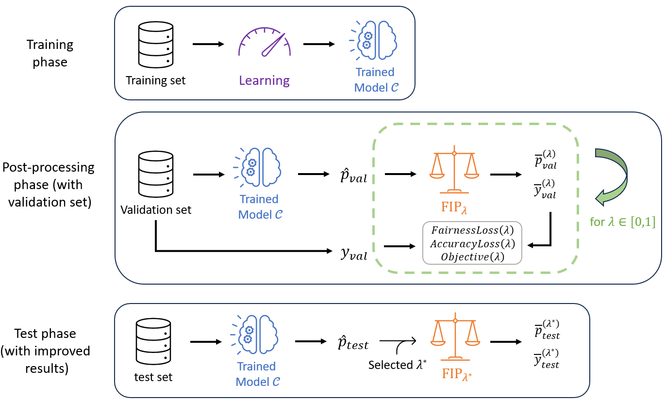
Our MADD post-processing method, illustrated in Figure 16, can be applied for a fixed \(\theta \)
as follows. Let us have a training, a validation and a test sets. We first train a classifier.
Then, we use this trained model on the validation set to output the predictions \(\hat {y}_{i,{validation}}\) and predicted
probabilities \(\hat {p}_{i,{validation}}\). Next, we apply our fip mapping function with various values of \(\lambda \) to obtain different
corresponding \(\overline {p}_{i,{validation}}^{(\lambda )}\). We will thus deduce the new \(\overline {y}_{i,{validation}}^{(\lambda )}\) thanks to the classification threshold \(t\). Now, with
the new \(\overline {p}_{i,{validation}}^{(\lambda )}\), \(\overline {y}_{i,{validation}}^{(\lambda )}\) and the true labels \(y_{i,{validation}}\), we can plot the results of our objective function depending
on the \(\lambda \)s to find the optimal \(\lambda ^{*}\) that will best improve the results of the classifier. Finally, we
evaluate the accuracy and the fairness of the results with the chosen \(\lambda ^{*}\) on the test set (i.e., with \(\overline {p}_{i,{test}}^{(\lambda ^*)})\), \(\overline {y}_{i,{test}}^{(\lambda ^{*})}\)
and the true labels \(y_{i,{test}}\)). For the sake of simplification, in the experiments we omit training,
validation and test subscripts from the notations, but they will be easily deduced from the
context.
6.2.2. Rescaled objective function
For our experiments, we use the objective function that we named \(\mathcal {L}_{exp}\) composed of the rescaled terms we define in Equations \eqref{eq:9}6 and \eqref{eq:10}. Notably, we multiply MADD by \(1/2\) for the term \(\operatorname {FairnessLoss}_{exp}\) to be in the same scale of the one of \(\operatorname {AccuracyLoss}_{exp}\). Therefore, both losses have a range of \([0, 100\%]\). The \(\operatorname {AccuracyLoss}_{exp}(\lambda )\) is the percentage of incorrect predictions, and the \(\operatorname {FairnessLoss}_{exp}(\lambda )\) now represents a percentage of dissimilarity between the two distributions. Thus, the resulting objective function \(\mathcal {L}_{exp}\) is a weighted average of these two losses based on their importance. However, as a case study, we choose to give, in all our experiments, the same importance both to the accuracy and the fairness in the post-processing, so we fix \(\theta = 0.5\). Additionally, it is important to note that in the case of this \(\operatorname {AccuracyLoss}_{exp}(\lambda )\), it exactly corresponds to 1 minus the standard accuracy score, which we will exploit in our results in Section 6.3. Our goal will be to experimentally find the optimal parameter \(\lambda ^*\) that minimizes this objective function \(\mathcal {L}_{exp}\), with \(\theta = 0.5\).
\begin {align} \operatorname {AccuracyLoss}_{exp}(\lambda ) &= \frac {1}{n} \sum _{i=1}^n \mathds {1}_{y_i \neq \overline {y}_i} \label {eq:9} \\ \operatorname {FairnessLoss}_{exp}(\lambda ) &= \frac {1}{2} \text {MADD}\left (\overline {D}_{G_0}, \overline {D}_{G_1}\right ) \label {eq:10} \end {align}
6.2.3. Simulated data
To demonstrate the validity of our approach, we first experiment with our MADD post-processing method on simulated data of \(\hat {p}_i\) for which we know the real distributions. We thus use the same simulated data that we presented in Section 4.4, and we refer the reader to this part for the details of how it has been generated.
Additionally to Section 4.4, we need here to simulate the true label \(y_i\) for each student \(i\). This will enable us to simulate how a classifier would perform before the post-processing, to compare its results with those obtained after the post-processing. The latter are thus deduced from the classification threshold parameter \(t\) that we set to 0.5 in this paper, and we refer the reader to the footnote 6. Thus, for the simulated \(y_i\), we arbitrarily choose to pass the simulated \(\hat {p}_i\) value as a parameter of a Bernoulli law: Bernoulli(\(\hat {p}_i\)) \(\in \left \{0, 1\right \}\).
6.2.4. Real-world educational data
As a second testbed for our approach, we use it with real-world educational data. Again, we use the data we already presented in Section 5. Since \(S = \text {poverty}\) obtained the highest MADD value in the course “BBB” (see Table 3), it is thus a relevant feature with respect to which it is interesting to improve fairness. It is worth noticing that as we split the data in a different way to have an additional validation set, it leads to slightly different distributions in the current test set from what was previously obtained.
6.3. Results
6.3.1. Simulated data
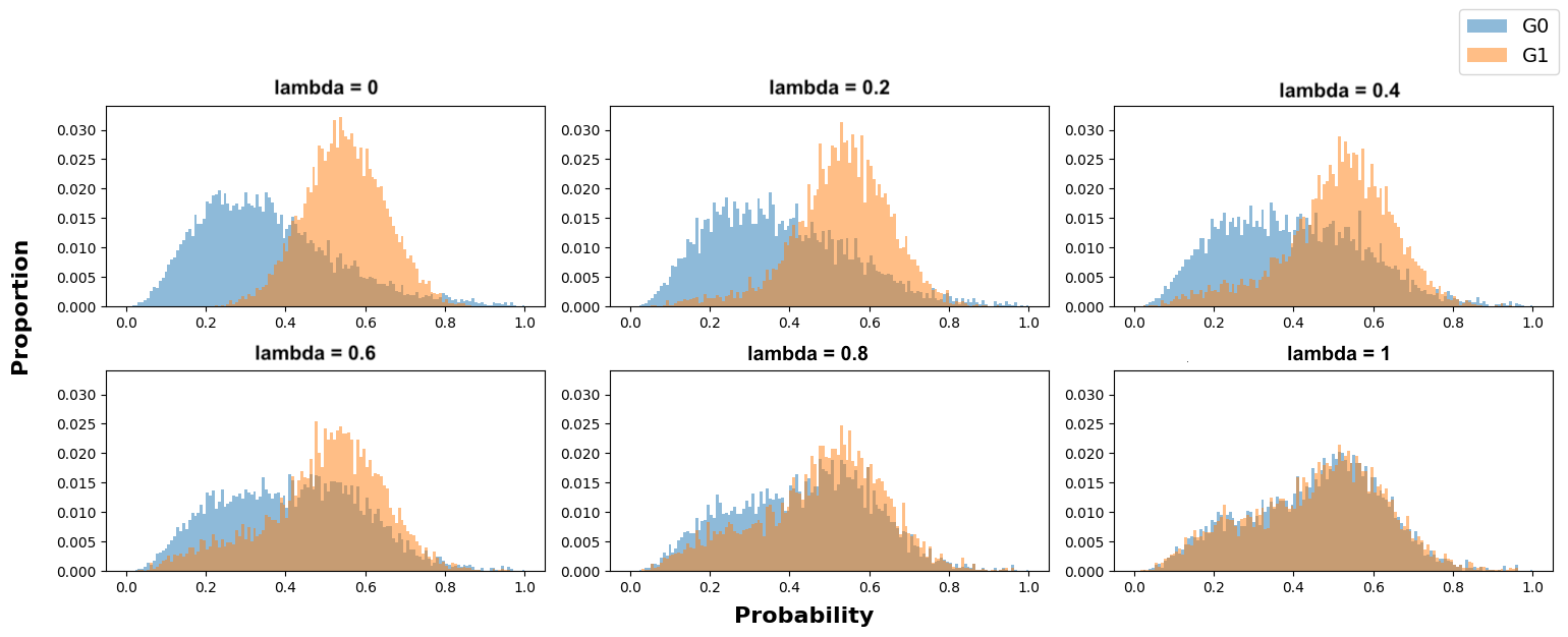
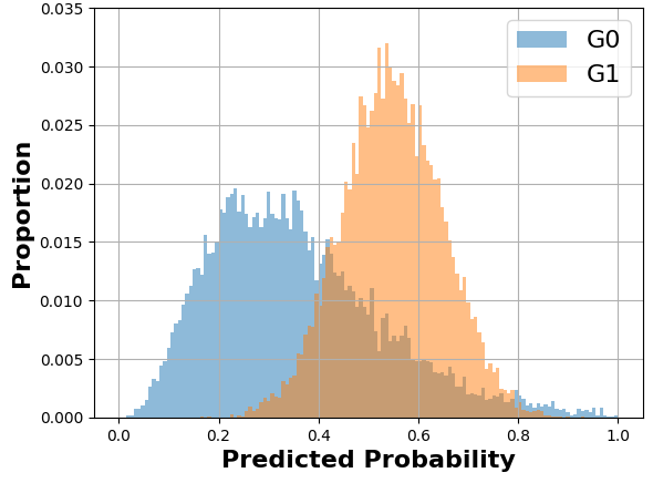
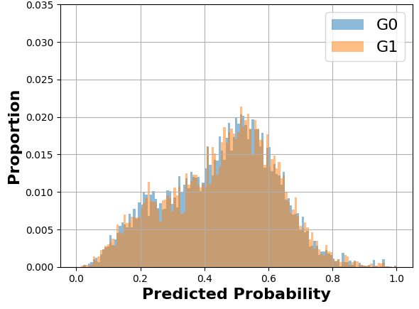
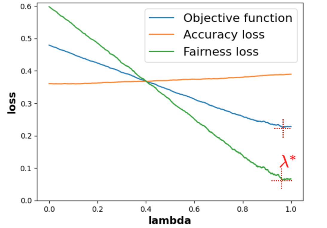
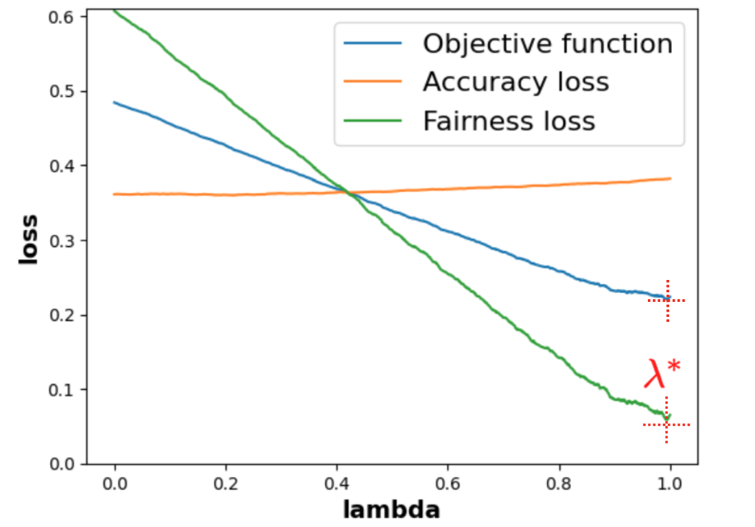
Figure 18: Simulated data results. (a) Histograms of \(D_{G_0}\) and \(D_{G_1}\) from simulated \(\hat {p}_{i \in G_0}\) and \(\hat {p}_{i \in G_1}\). (b) Histograms of the new \(\overline {D}_{G_0}\) and \(\overline {D}_{G_1}\). (c, d) Objective function (total loss), accuracy loss and fairness loss.
We generate \(1,000\) values of \(\lambda \) with a constant step in its interval \([0,1]\), and then we compute all the
corresponding \(\overline {p}_i(\lambda )\), in order to obtain the relationships between the next three \(\mathcal {L}_{exp}\), \(\operatorname {AccuracyLoss}_{exp}(\lambda )\), \(\operatorname {FairnessLoss}_{exp}(\lambda )\) and \(\lambda \). In Figure 17, we
present how the new predicted probabilities progress with some increasing values of \(\lambda \). In Figure 17c,
we display for all values of \(\lambda \) the evolution of \(\mathcal {L}_{exp}\), \(\operatorname {AccuracyLoss}_{exp}(\lambda )\) and \(\operatorname {FairnessLoss}_{exp}(\lambda )\). We remind that we set \(\theta = 0.5\) as we decided to give equal
importance to both the accuracy and the fairness in the post-processing. As we can see in Figure 17c,
on the one hand, when \(\lambda \) increases, the accuracy loss increases too (while we want to minimize it), but
only slightly (\(0.361\) to \(0.390\), i.e., about +\(8\)%). On the other hand, the fairness loss, which corresponds to
half of MADD, significantly drops as what we look for (\(0.598\) to its lowest at \(0.063\), i.e. about -\(90\)%). In
addition, the objective function \(\mathcal {L}_{exp}\) reaches its minimum value \(0.226\) at \(\lambda ^{*} = 0.970\), almost 1. Therefore, if we
accept to lose about \(8\)% of accuracy (we can make this interpretation because of how we
defined our \(\operatorname {AccuracyLoss}_{exp}(\lambda )\)), then by choosing \(\lambda ^{*} = 0.970\), we would increase the fairness of the results by \(90\)% w.r.t the
MADD criterion. After that, we only have to pass \(\lambda ^{*} = 0.970\) and the \(\hat {p}_i\) as inputs of fip to obtain our new
fairer predicted probabilities as shown in Figure 17b. We have repeated the simulation by
generating some other random \(10,000\) samples for each group, and the results are very similar
(see Figure 17d), which strengthens the estimation of \(\lambda ^{*}\) being close to \(1\). To conclude, this
experiment, based on a simulated and ideal case study with sufficient data, demonstrates that the
MADD post-processing manages to preserve a reasonably similar level of accuracy while
significantly improving the fairness of the results. Let us now apply it to real-world data in the next
part.
6.3.2. Real-world educational data
Similarly to what was done in the previous section, we display in Figure 18c the evolution of \(\mathcal {L}_{exp}\), \(\operatorname {AccuracyLoss}_{exp}(\lambda )\) and \(\operatorname {FairnessLoss}_{exp}(\lambda )\), for the values of \(\lambda \) we generated in part 6.3.1. When \(\lambda \) increases, the accuracy loss remains almost constant (\(0.332\) to \(0.336\) i.e. about +1%), and the fairness loss significantly drops again (\(0.431\) to its lowest at \(0.158\), i.e. about \(-63\%\)). However, Figure 18c shows a lot more variability than in the previous case study, which comes from the much lower number of samples in the validation set (about \(700\)). This loss in precision makes it more challenging to find an optimal \(\lambda ^{*}\). Indeed, we see that the minimum of the objective function (\(0.241\)) is not necessarily reached at the optimal \(\lambda ^{*}\) (\(0.798\)) because the \(\operatorname {FairnessLoss}(\lambda )\) seems to keep decreasing but the computation is not precise enough. Nonetheless, we select this \(\lambda ^{*} = 0.798\) value to visually evaluate how close or far the results are from satisfying fairness. We can still observe satisfying results from Figures 18a to 18b. To conclude, similarly to ML in general, the MADD post-processing is sensitive to the number of data, but it still shows very successful fairness improvement without losing too much accuracy of the results.
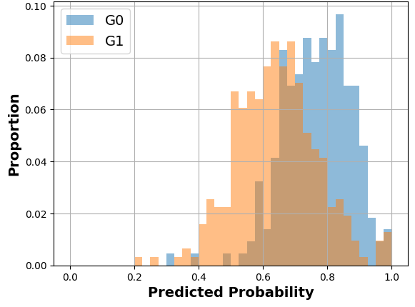
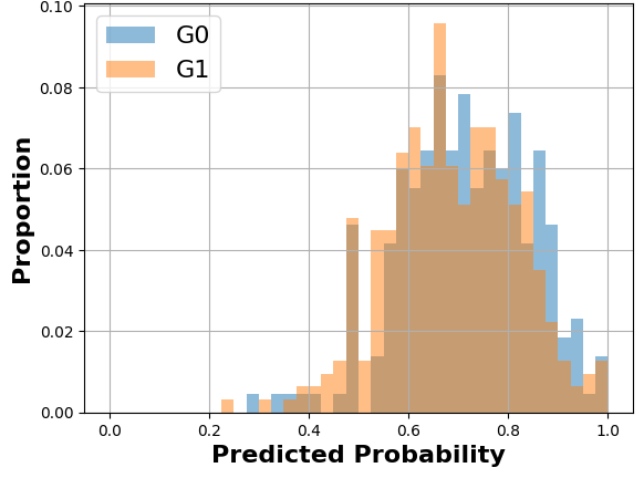
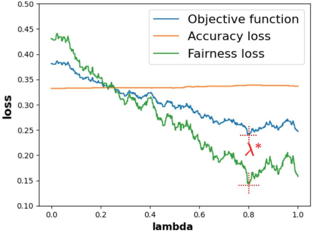
Figure 19: Real-world educational data results.
6.4. Influence of the number of samples
Moreover, thanks to our definition of the post-processing method, the fairness of the improved estimated probabilities is predictable. Indeed, the MADD of the improved estimated probabilities, \(\text {MADD}\left (\overline {D}_{G_0}, \overline {D}_{G_1}\right )\), is a function of \(\lambda \) that converges when the sample size \(n\) increases to \((1 - \lambda ) \cdot \text {MADD}\left ({D}_{G_0}, {D}_{G_1}\right )\). This means that, for any selected \(\lambda \), after post-processing, its new MADD value approximates \((1 - \lambda )\) times the old MADD value, and the larger the sample size \(n\), the more accurate this estimate is. This property is shown in Figure 20: the \(\text {MADD}\left (\overline {D}_{G_0}, \overline {D}_{G_1}\right )\) function converges to the function \((1 - \lambda ) \text {MADD}\left ({D}_{G_0}, {D}_{G_1}\right ) \) as the sample size increases.
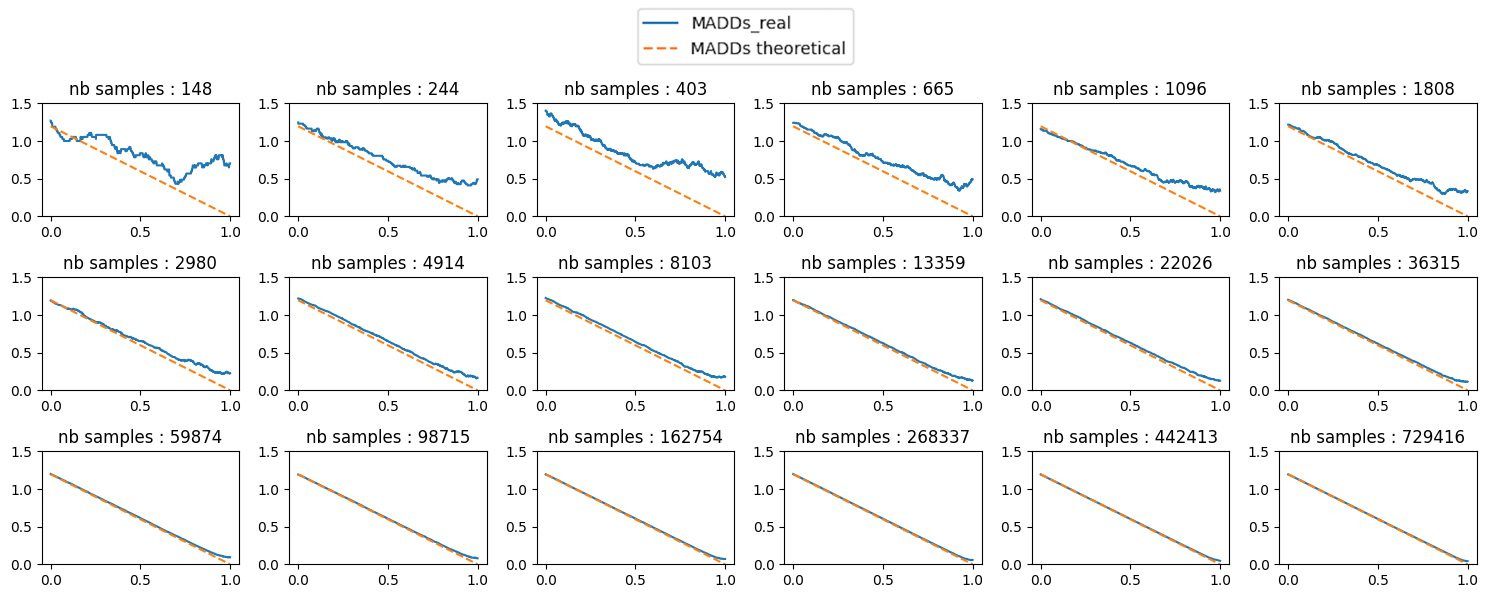
7. Discussion
We now discuss the main implications of our work regarding (1) the MADD metric itself, (2) the fairness evaluation with MADD, and (3) the MADD post-processing.
Firstly, the strengths of MADD consist in taking into account the entire predicted probability distributions compared to existing metrics, and handling any of their forms. It is also an easily interpretable fairness metric, enabling visual analyses through the plot of the two related distributions. On the other hand, a major limitation of MADD in its original version was its sensitivity to its bandwidth parameter (\(h\)) and to the number of samples (\(n\)) contained in a dataset. In this paper, we provided theoretical guarantees and an automated search algorithm to alleviate this issue, by finding optimal bandwidths for which MADD best estimates algorithmic unfairness. This is an important contribution as it ensures the robustness of MADD. Regarding the choice of standard deviation in the automated search algorithm, any other variation metric would have given the same result, since we are looking for the interval where MADD is stable, relatively over the search space, and since any optimal \(h\), and not a single one, is valid in this interval.
In future work, we aim to apply MADD to other educational datasets and predictive tasks, so as to
further assess fairness in other contexts. In line with this, we provided a Python package, maddlib3,
so that other researchers and developers can replicate, assess, and mitigate the fairness of their results
with this metric. Also, MADD currently works for binary groups and binary prediction classes, which,
as said in the introduction, is suitable in many cases as it corresponds in practice to the
main prediction tasks in education. While focusing on binary information has advantages,
including the fact that it makes it possible to plot and interpret MADD easily, other relevant
applications of predictive models in education are not binary, which could be addressed in future
work.
Secondly, regarding fairness evaluation with MADD, we saw that this metric best estimates the distance between the distributions of two groups when \(h\) is carefully chosen into its optimal interval. These optimal \(h\) values mostly depend on the numbers of students belonging to both groups, \(n_0\) and \(n_1\), as explained in Section 4.2. This has two important consequences. First, the optimal interval should be computed for each feature with respect to which we want to evaluate algorithmic unfairness and more specifically for each measurement (model-feature combination). Second, two MADD values should be compared only if they have been computed with an optimal \(h\), otherwise there is no guarantee that both of these values had converged. For instance, if we assume that a given sensitive feature (e.g., gender) leads to a MADD score of \(1.5\) with a model \(\mathcal {M}_1\) trained on a dataset \(d_1\), and a score of \(0.5\) with a model \(\mathcal {M}_2\) trained on a dataset \(d_2\), then we can say that the first setting is more discriminant with regards to this sensitive feature than the second one, provided that MADD was calculated with an optimal \(h\) in both cases.
Although it is essential to choose the right bandwidth \(h\), it is worth emphasizing that performing a
fairness evaluation with MADD does not prevent from evaluating the predictive performance of the
models as well. Indeed, as mentioned in (Verger et al., 2023), a model that shows poor
predictive performance is not necessarily behaving unfairly regarding the studied groups, but it would
then be unable to make relevant predictions for the success or failure of students for instance,
which makes this model not usable in practice. We refer the reader to Section 5.2 of (Verger
et al., 2023) for a comparison with a predictive-performance oriented fairness
metric, ABROCA (Gardner et al., 2019), and the main related takeaways
in part 5.2.3. Furthermore, an extension of MADD would be to generalize its definition
(Equation \eqref{MADDeq}) to take into account the influence of several features on the fairness
evaluation, which is scarcely studied in the literature. Several possibilities exist and will be further
studied in future work.
Thirdly, regarding the mitigation with MADD through post-processing, its performance depends on
the number of samples \(n_0\) and \(n_1\), too. Indeed, the more precise both distributions are, the more likely it is
that the new fairer distributions will reach the target distribution as precisely as possible. Granted that
there is sufficient data, we found that our method can successfully improve the fairness of the results
regarding two groups, without losing too much accuracy. While there is a need to replicate this finding,
it is noteworthy that we could improve the MADD values of some results by up to \(63\)% with real-world
data.
Overall, even if, with MADD or any other metric, we seek to best estimate algorithmic unfairness
and mitigate it, these fairness metrics cannot be the only way to assess the fairness of a system meant
to improve the learning experience or to assist decision making. Indeed, fairness should
be considered as a global notion including the system, with all its components (e.g., data,
models, interfaces), but also its multiple stakeholders (e.g., institutions, students, instructors,
developers, researchers – see Romero and Ventura (2020), Holstein and Doroudi (2021) for a
complete list of them in an educational context – but also policymakers, lawyers, sociologists,
philosophers, etc.). Calvi and Kotzinos (2023) thus paves the way towards a global framework to
reach a higher level of evaluation through an algorithmic impact assessment (AIA) of the
systems. AIAs are meant to be iterative processes used to investigate the possible short and
long-term societal impacts of AI systems before their use, but with ongoing monitoring and
periodic revisiting even after their implementation. Nonetheless, fairness metrics are so far the
most advanced techniques available to evaluate algorithmic fairness (Calvi and Kotzinos,
2023).
8. Conclusion
In this paper, we focused on Model Absolute Density Distance (MADD), a fairness metric we recently proposed (Verger et al., 2023) to measure predictive models’ discriminatory behaviors between groups. This metric is based on comparing the probability distributions outputted by the models for each group, to uncover and measure the difference in these distributions that could reveal unfair predictions.
Specifically, in this paper, we contributed to the work of Verger et al. (2023) in three
ways. First, we provide a more rigorous definition of the MADD metric, based on the mathematical
properties of histogram estimators. This allowed us to provide an algorithm for automatically
optimizing the bandwidth, i.e., the MADD hyperparameter, which in our previous work was arbitrarily
set to a predefined default value (Verger et al., 2023). Second, we provide a method that
leverages MADD to mitigate the algorithmic unfairness of a model without hindering its accuracy, via
post-processing of the probability distributions produced by the model. Third, we developed an
open-source Python package named maddlib3 to facilitate the usage of MADD in future
work.
To evaluate our work, we conducted experiments with both simulated and real-world educational data. In particular, the real-world data came from two online courses, and we studied the fairness of ML classifiers which predicted whether students would pass or fail courses, depending on their demographics and interactions with the course material. Our results did show that trained on the same data, models exhibit different discriminatory behaviors according to different sensitive features, thus generating different levels of unfair predictions. Furthermore, there is no direct relationship between the bias that already exists in the data and the algorithmic unfairness of the models. For instance, we found that in a course, several models exhibited more unfair behaviors for students based on their poverty, whereas the data were actually heavily skewed for gender and disability features (Verger et al., 2023).
Our results show that we can successfully and substantially mitigate the unfair behaviors of the models with our MADD-based post-processing method, without hindering accuracy. This finding is promising for the value of our mitigation approach. The data and code of our experiments are publicly available (see Section 1).
For future work, we plan to further study the value of MADD with other datasets. We also plan to target other predictive tasks commonly used in education, such as predicting students at risk of dropping out of a course, predicting skill acquisition, or predicting scholarship acceptance. As for the MADD metric, we aim to extend it to take into account combinations of features that could generate more unfair predictions than each feature taken separately. This is crucial to account for the fact that membership in several groups can result in unique combinations of discrimination, known as intersectional discrimination. To the best of our knowledge, such studies are still lacking in education, and we initiate a work in this direction.
9. Acknowledgements
This work was supported by Sorbonne Center for Artificial Intelligence (SCAI), and Direction du Numérique Educatif (DNE) of the French Ministry of Education. The views and opinions expressed in this manuscript are those of the authors and do not necessarily reflect those of SCAI and DNE.
References
- Anderson, H., Boodhwani, A., and Baker, R. 2019. Assessing the Fairness of Graduation Predictions. In Proceedings of The 12th International Conference on Educational Data Mining (EDM), C. F. Lynch, A. Merceron, M. Desmarais, and R. Nkambou, Eds. International Educational Data Mining Society, Montreal, Canada, 488–491.
- Baker, R. S., Esbenshade, L., Vitale, J., and Karumbaiah, S. 2023. Using Demographic Data as Predictor Variables: a Questionable Choice. Journal of Educational Data Mining (JEDM) 15, 2 (Jun.), 22–52.
- Baker, R. S. and Hawn, A. 2021. Algorithmic Bias in Education. International Journal of Artificial Intelligence in Education (IJAIED) 32, 4 (Nov.), 1052–1092.
- Barocas, S., Hardt, M., and Narayanan, A. 2019. Fairness and Machine Learning: Limitations
and Opportunities. MIT Press, Cambridge, MA.
http://www.fairmlbook.org. - Bolukbasi, T., Chang, K.-W., Zou, J., Saligrama, V., and Kalai, A. 2016. Man is to Computer Programmer as Woman is to Homemaker? Debiasing Word Embeddings. In Proceedings of the 30th Conference on Neural Information Processing Systems (NIPS 2016), D. D. Lee, M. Sugiyama, U. von Luxburg, I. Guyon, and R. Garnett, Eds. Curran Associates Inc., Barcelona, Spain, 4356––4364.
- Buolamwini, J. and Gebru, T. 2018. Gender Shades: Intersectional Accuracy Disparities in Commercial Gender Classification. In Proceedings of the 1st Conference on Fairness, Accountability and Transparency (ACM FAccT,). Proceedings of Machine Learning Research, vol. 81. PMLR, New York, NY, USA, 77–91.
- Calvi, A. and Kotzinos, D. 2023. Enhancing AI fairness through impact assessment in the European Union: a legal and computer science perspective. In Proceedings of the 6th Conference on Fairness, Accountability, and Transparency (ACM FAccT). Association for Computing Machinery, Chicago, IL, USA, 1229–1245.
- Castelnovo, A., Crupi, R., Greco, G., Regoli, D., Penco, I. G., and Cosentini, A. C. 2022. A clarification of the nuances in the fairness metrics landscape. Scientific Reports 12, 1–21. Nature Publishing Group.
- Caton, S. and Haas, C. 2024. Fairness in Machine Learning: A Survey. ACM Computing Surveys 56, 7 (Apr.), 1–38.
- Cha, S.-H. and Srihari, S. N. 2002. On measuring the distance between histograms. Pattern Recognition 35, 1355–1370.
- Christie, S. T., Jarratt, D. C., Olson, L. A., and Taijala, T. T. 2019. Machine-Learned School Dropout Early Warning at Scale. In Proceedings of The 12th International Conference on Educational Data Mining (EDM), C. F. Lynch, A. Merceron, M. Desmarais, and R. Nkambou, Eds. International Educational Data Mining Society, Montreal, Canada, 726–731.
- d’Alessandro, B., O’Neil, C., and LaGatta, T. 2017. Conscientious Classification: A Data Scientist’s Guide to Discrimination-Aware Classification. Big Data 5, 2 (Jun.), 120–134.
- Dastin, J. 2018. Amazon scraps secret AI recruiting tool that showed bias against women. Reuters.
https://www.reuters.com/article/us-amazon-com-jobs-automation-insight-idUSKCN1MK08G. - Deho, O. B., Zhan, C., Li, J., Liu, J., Liu, L., and Duy Le, T. 2022. How do the existing fairness metrics and unfairness mitigation algorithms contribute to ethical learning analytics? British Journal of Educational Technology 53, 4, 822–843.
- Devroye, L. 1986. Non-Uniform Random Variate Generation. Springer, New York, NY.
- Devroye, L. and Gyorfi, L. 1985. Nonparametric Density Estimation: The L1 View. In Wiley Series
in Probability and Statistics. John Wiley and Sons, New York.
https://www.szit.bme.hu/˜gyorfi/L1bookBW.pdf. - Gardner, J., Brooks, C., and Baker, R. 2019. Evaluating the Fairness of Predictive Student Models Through Slicing Analysis. In Proceedings of the 9th International Conference on Learning Analytics & Knowledge. ACM, Tempe AZ USA, p. 225–234.
- Holstein, K. and Doroudi, S. 2021. Equity and Artificial Intelligence in Education: Will “AIEd” Amplify or Alleviate Inequities in Education? CoRR abs/2104.12920.
- Hu, Q. and Rangwala, H. 2020. Towards Fair Educational Data Mining: A Case Study on Detecting At-risk Students. In Proceedings of the 13th International Conference on Educational Data Mining (EDM), A. N. Rafferty, J. Whitehill, V. Cavalli-Sforza, and C. Romero, Eds. International Educational Data Mining Society, Fully virtual, 431–437.
- Hutchinson, B. and Mitchell, M. 2019. 50 Years of Test (Un)fairness: Lessons for Machine Learning. In Proceedings of the 2nd Conference on Fairness, Accountability, and Transparency (ACM FAccT). Association for Computing Machinery, Atlanta GA USA, 49–58.
- Hutt, S., Gardner, M., Duckworth, A. L., and D’Mello, S. K. 2019. Evaluating Fairness and Generalizability in Models Predicting On-Time Graduation from College Applications. In Proceedings of the 12th International Conference on Educational Data Mining (EDM), C. F. Lynch, A. Merceron, M. Desmarais, and R. Nkambou, Eds. International Educational Data Mining Society, Montreal, Canada, 79–88.
- Jiang, W. and Pardos, Z. A. 2021. Towards Equity and Algorithmic Fairness in Student Grade Prediction. In Proceedings of the 2021 AAAI/ACM Conference on AI, Ethics, and Society, I. Roll, D. McNamara, S. Sosnovsky, R. Luckin, and V. Dimitrova, Eds. Association for Computing Machinery, New York, NY, USA, 608––617.
- Kai, S., Andres, J. M. L., Paquette, L., Baker, R. S., Molnar, K., Watkins, H., and Moore, M. 2017. Predicting Student Retention from Behavior in an Online Orientation Course. In Proceedings of the 10th International Conference on Educational Data Mining (EDM), X. Hu, T. Barnes, A. Hershkovitz, and L. Paquette, Eds. International Educational Data Mining Society, Wuhan, Hubei, China.
- Kizilcec, R. F. and Lee, H. 2022. Algorithmic Fairness in Education. In Ethics in Artificial Intelligence in Education, W. Holmes and K. Porayska-Pomsta, Eds. Taylor & Francis, New York.
- Kuzilek, J., Hlosta, M., and Zdrahal, Z. 2017. Open University Learning Analytics dataset. Scientific data 4, 1, 1–8.
- Lallé, S., Bouchet, F., Verger, M., and Luengo, V. 2024. Fairness of MOOC Completion Predictions Across Demographics and Contextual Variables. In Proceedings of the 25th International Conference on Artificial Intelligence in Education (AIED). Springer, Recife, Brazil. In press.
- Larson, J., Mattu, S., Kirchner, L., and Angwin, J. 2016.
How We Analyzed the COMPAS Recidivism Algorithm. ProPublica.
https://www.propublica.org/article/how-we-analyzed-the-compas-recidivism-algorithm. - Le Quy, T., Roy, A., Iosifidis, V., Zhang, W., and Ntoutsi, E. 2022. A survey on datasets for fairness-aware machine learning. WIREs Data Mining and Knowledge Discovery 12, 3, e1452.
- Lee, H. and Kizilcec, R. F. 2020. Evaluation of Fairness Trade-offs in Predicting Student Success.
FATED (Fairness, Accountability, and Transparency in Educational Data) Workshop at EDM 2020.
https://doi.org/10.48550/arXiv.2007.00088. - Li, C., Xing, W., and Leite, W. 2021. Yet another predictive model? Fair predictions of students’ learning outcomes in an online math learning platform. In Proceedings of the 11th International Learning Analytics and Knowledge Conference. Association for Computing Machinery, Irvine, CA, USA, 572–578.
- Lopez, P. 2021. Bias does not equal bias: a socio-technical typology of bias in data-based algorithmic systems. Internet Policy Review 10, 4 (Dec.), 1–29.
- Makhlouf, K., Zhioua, S., and Palamidessi, C. 2021. Machine learning fairness notions: Bridging the gap with real-world applications. Information Processing & Management 58, 5 (Sep.), 102642.
- Mehrabi, N., Morstatter, F., Saxena, N., Lerman, K., and Galstyan, A. 2022. A Survey on Bias and Fairness in Machine Learning. ACM Computing Surveys 54, 6, 1–35.
- Pessach, D. and Shmueli, E. 2023. Algorithmic Fairness. In Machine Learning for Data Science Handbook: Data Mining and Knowledge Discovery Handbook, L. Rokach, O. Maimon, and E. Shmueli, Eds. Springer, Cham, Switzerland, 867–886.
- Romero, C. and Ventura, S. 2020. Educational data mining and learning analytics: An updated survey. Wiley Interdisciplinary Reviews: Data Mining and Knowledge Discovery 10, 3, e1355.
- Selbst, A. D., Boyd, D., Friedler, S. A., Venkatasubramanian, S., and Vertesi, J. 2019. Fairness and Abstraction in Sociotechnical Systems. In Proceedings of the 2nd Conference on Fairness, Accountability, and Transparency (ACM FAccT). Association for Computing Machinery, Atlanta GA USA, 59–68.
- Sha, L., Rakovic, M., Whitelock-Wainwright, A., Carroll, D., Yew, V. M., Gasevic, D., and Chen, G. 2021. Assessing algorithmic fairness in automatic classifiers of educational forum posts. In Proceedings of the 22nd International Conference on Artificial Intelligence in Education (AIED), I. Roll, D. McNamara, S. Sosnovsky, R. Luckin, and V. Dimitrova, Eds. Springer, Utrecht, The Netherlands, 381–394.
- Sovrano, F., Sapienza, S., Palmirani, M., and Vitali, F. 2022. A Survey on Methods and Metrics for the Assessment of Explainability under the Proposed AI Act. In Legal Knowledge and Information Systems: JURIX 2021: The Thirty-fourth Annual Conference, E. Schweighofer, Ed. IOS Press, Vilnius, Lithuania, 235–242.
- Suresh, H. and Guttag, J. V. 2021. A Framework for Understanding Sources of Harm throughout the Machine Learning Life Cycle. In Proceedings of the 1st ACM Conference on Equity and Access in Algorithms, Mechanisms, and Optimization. Association for Computing Machinery, New York, NY, USA, 1–9.
- Vasquez Verdugo, J., Gitiaux, X., Ortega, C., and Rangwala, H. 2022. FairEd: A Systematic Fairness Analysis Approach Applied in a Higher Educational Context. In LAK22: 12th International Learning Analytics and Knowledge Conference. Association for Computing Machinery, Online USA, 271–281.
- Verger, M., Lallé, S., Bouchet, F., and Luengo, V. 2023. Is Your Model “MADD”? A Novel Metric to Evaluate Algorithmic Fairness for Predictive Student Models. In Proceedings of the 16th International Conference on Educational Data Mining, M. Feng, T. Käser, and P. Talukdar, Eds. International Educational Data Mining Society, Bengaluru, India, 91–102.
- Verma, S. and Rubin, J. S. 2018. Fairness Definitions Explained. In Proceedings of the 2018 IEEE/ACM International Workshop on Software Fairness (FairWare). Association for Computing Machinery, Gothenburg Sweden, 1–7.
- Yu, R., Lee, H., and Kizilcec, R. F. 2021. Should college dropout prediction models include protected attributes? In Proceedings of the Eighth ACM Conference on Learning @ Scale. L@S ’21. Association for Computing Machinery, New York, NY, USA, p. 91–100.
- Yu, R., Li, Q., Fischer, C., Doroudi, S., and Xu, D. 2020. Towards accurate and fair prediction of college success: Evaluating different sources of student data. In Proceedings of The 13th International Conference on Educational Data Mining (EDM), A. N. Rafferty, J. Whitehill, V. Cavalli-Sforza, and C. Romero, Eds. International Educational Data Mining Society, Fully virtual, 292–301.
- Švábenský, V., Verger, M., Rodrigo, M. M. T., Monterozo, C. J. G., Baker, R. S., Saavedra, M. Z. N. L., Lallé, S., and Shimada, A. 2024. Evaluating Algorithmic Bias in Models for Predicting Academic Performance of Filipino Students. In Proceedings of The 17th International Conference on Educational Data Mining (EDM). International Educational Data Mining Society, Atlanta, Georgia, USA. In press.
10. Appendices
10.1. Proof of Theorem 1
Proof. To prove the theorem, we start from the definition of MADD (Equation 3) and the properties of the indicator function (noted \(\mathds {1}\) and defined in Equation \eqref{indicatorUNDERSCOREfunctionUNDERSCOREeq}). Specifically, we have:
\[ \begin {aligned} &\operatorname {MADD}\left (D_{G_0}, D_{G_1}\right ) \\ := &\sum _{k=1}^m\left | d_{G_0, k} - d_{G_1, k} \right | \\ &\text {by definition of $d_{G_0, k}$ and $d_{G_1, k}$ in Equation~\eqref {d-k-def}:}\\ = &\sum _{k=1}^m \left | \frac {1}{n_0} \sum _{i=1}^{n_0} \mathds {1}_{I_k}\left ( \hat {p}_i^{(0)} \right ) - \frac {1}{n_1} \sum _{i=1}^{n_1} \mathds {1}_{I_k}\left ( \hat {p}_i^{(1)} \right ) \right |\\ &\text {by calculating the integral thanks to the definition of the indicator function:}\\ = &\int _0^1 \frac {1}{h} \sum _{k=1}^m \left | \frac {1}{n_0} \sum _{i=1}^{n_0} \mathds {1}_{I_k}\left ( \hat {p}_i^{(0)} \right ) - \frac {1}{n_1} \sum _{i=1}^{n_1} \mathds {1}_{I_k}\left ( \hat {p}_i^{(1)} \right ) \right | \mathds {1}_{I_k}(x) dx\\ &\text {by distributing the indicator function:}\\ =&\int _0^1 \left |\frac {1}{h} \sum _{k=1}^m \left ( \frac {1}{n_0} \sum _{i=1}^{n_0} \mathds {1}_{I_k}\left ( \hat {p}_i^{(0)} \right ) \right ) \mathds {1}_{I_k}(x) - \frac {1}{h} \sum _{k=1}^m \left ( \frac {1}{n_1} \sum _{i=1}^{n_1} \mathds {1}_{I_k}\left ( \hat {p}_i^{(1)} \right ) \right ) \mathds {1}_{I_k}(x) \right | dx \\ &\text {by definition of histogram function (Definition 1):}\\ =&\int _0^1 \left |\widehat {f}^{G_0}_h(x) - \widehat {f}^{G_1}_h(x) \right | dx \\ &\text {by definition of } L_1 \text { distance (Definition 2):}\\ = &\left \|\widehat {f}^{G_0}_h(x) - \widehat {f}^{G_1}_h(x)\right \|_{L_1[0,1]} \end {aligned} \]
10.2. Proof of Theorem 2
We first clarify the conditions required for Theorem 2 to be held. Let us introduce \(\mathcal {F}\), the class of functions satisfying the following conditions for any function \(\xi \in \mathcal {F}\):
-
\(\xi \) has compact support,
-
\(\xi \) is absolutely continuous with derivative \(\xi ^{\prime }\) almost everywhere,
-
\(\xi ^{\prime }\) is bounded and continuous.
Thus, we assume that both PDFs \(f^{G_0}, f^{G_1} \in \mathcal {F}\). Indeed, the first condition is necessarily satisfied since, in our case, the model gives predicted probabilities that are continuous-valued in \([0,1]\) (compact support), and the two other conditions, which are smoothness assumptions, are generally regarded as standard and relatively undemanding requirement in continuous-valued non-parametric estimation (Devroye and Gyorfi, 1985).
Before going into the details of Theorem 2, we introduce some necessary notions. In statistics, the risk often represents the mathematical expectation of the absolute quadratic error between an estimator and its target. Here, the error is the difference between MADD and the true \(\left \| f^{G_0} - f^{G_1} \right \|_{L_1[0,1]}\). The reason for finding the expectation of this difference is that the samples are random, so the value of MADD will be different for different samples. Thus, the risk of an estimator represents its theoretical mean error. Therefore, we define the risk as follows:
Definition 3 (Risk). \begin {align*} &\mathcal {R}\left ( \operatorname {MADD}\left (D_{G_0}, D_{G_1}\right ), \left \| f^{G_0} - f^{G_1} \right \|_{L_1[0,1]} \right ) \\ := &\ \mathbb {E}\left [ \left | \operatorname {MADD}\left (D_{G_0}, D_{G_1}\right ) - \left \| f^{G_0} - f^{G_1} \right \|_{L_1[0,1]} \right | \right ] \end {align*}
For a good estimator, this risk should converge to 0 when the number of samples converges to infinity. Nonetheless, in general, we also need to know how quickly it converges to 0. For example, if the risk of one estimator is \(1/n\), and the risk of another estimator is \(1/n^2 + 1/n^3\), we should choose the second one, even if when \(n=1\), the first risk is smaller than the second, because the second risk converges to 0 more quickly, which means that when \(n\) is sufficiently large, the second risk will be much smaller than the first one. Now, we define the convergence speed formally:
Definition 4 (Convergence speed). For an estimator \(\widehat {\xi }\) and its risk \(\mathcal {R}\left (\widehat {\xi }, \xi \right )\), if there exists a constant \(C>0\) and a positive function \(\psi (n)\) such that \[ \limsup _{n \rightarrow +\infty } \psi (n) \mathcal {R}\left (\widehat {\xi }, \xi \right )=C \] i.e., \(\mathcal {R}\left (\widehat {\xi }, \xi \right ) = O \left ( \psi (n)^{-1} \right )\), then the convergence rate of \(\widehat {\xi }\) is said to be at least of order \(\psi (n)^{-1}\).
Then, for an estimator which needs a parameter \(h\) dynamically chosen according to \(n\), we define the optimal convergence speed as follows:
Definition 5 (Optimal convergence speed). For an estimator \(\widehat {\xi }_h\) and its risk \(\mathcal {R}\left (\widehat {\xi }_h, \xi \right )\), if there exists a constant \(C>0\) and a positive function \(\psi (n)\) such that \[ \limsup _{n \rightarrow +\infty } \inf _{h} \psi (n) \mathcal {R}\left (\widehat {\xi }_h, \xi \right )=C \] then the optimal convergence rate of \(\widehat {\xi }_h\) is said to be at least of order \(\psi (n)^{-1}\).
We also clarified the two following definitions.
Definition 6 (Asymptotic speed upper bound). Let a \(\in \mathbb {R}\). For two functions \(f\) and \(g\), if \(\exists d>0, C>0, \forall x \text { s.t }. |x-a|<d \Rightarrow |f(x)| \leq C|g(x)|\), then we denote \[ f(x)=\underset {x \rightarrow a}{O}(g(x)) \] If \(g\) is non-zero in the neighbourhood of \(a\), is equivalent to say \[ \limsup _{x \rightarrow a}\left |\frac {f(x)}{g(x)}\right |<\infty \]
Definition 7 (Asymptotically negligible). For two positive functions \(f\) and \(g\), if \(\displaystyle \lim _{x \rightarrow a} \frac {f(x)}{g(x)} = 0\), then we denote \[ f(x)=\underset {x \rightarrow a}{o}(g(x)) \] We can say that \(f\) is negligible compared to \(g\). When the context is clear, the subscript \(x \rightarrow a\) below \(O\) and \(o\) can be omitted.
We can now propose a mathematically rigorous version of Theorem 2 as follows using Definition 5:
Theorem 2 (Complete version)_____________________________
If \(f^{G_0}, f^{G_1} \in \mathcal {F}\), then \(\text {MADD}\left (D_{G_0}, D_{G_1}\right )\) converges to \(\left \| f^{G_0} - f^{G_1} \right \|_{L_1[0,1]}\) in the sense of the risk in \(L_1\), with an optimal convergence speed of at least \(\left ( \frac {\sqrt {n_0} + \sqrt {n_1} }{ \sqrt {n_0 n_1}} \right )^{\frac {2}{3}}\), i.e. \(\exists C>0\) : \begin {equation} \label {eq:cv_rate} \limsup _{\substack {n_0 \rightarrow +\infty \\ n_1 \rightarrow +\infty }} \inf _h \left ( \frac {\sqrt {n_0} + \sqrt {n_1} }{ \sqrt {n_0 n_1}} \right )^{-\frac {2}{3}} \mathbb {E}\left [ \left | \operatorname {MADD}\left (D_{G_0}, D_{G_1}\right ) - \left \| f^{G_0} - f^{G_1} \right \|_{L_1[0,1]} \right | \right ] = C \end {equation} where \(D_{G_0}\) and \(D_{G_0}\) depend on \(h\). This speed is reached when \(h=O\left (\left ( \frac {\sqrt {n_0} + \sqrt {n_1} }{ \sqrt {n_0 n_1}} \right )^{\frac {2}{3}}\right )\).
_________
Proof. To establish the theorem, we begin by examining the \(L_1\) difference between \(f^{G_0} - f^{G_1}\) and \(\widehat {f}^{G_0}_h - \widehat {f}^{G_1}_h\):
\[ \begin {aligned} &\left \| \left ( f^{G_0} - f^{G_1} \right ) - \left ( \widehat {f}^{G_0}_h - \widehat {f}^{G_1}_h \right ) \right \|_{L_1} \\ = &\left \| \left ( f^{G_0} - \widehat {f}^{G_0}_h \right ) - \left ( f^{G_1} - \widehat {f}^{G_1}_h \right ) \right \|_{L_1} \\ \leq &\left \| f^{G_0} - \widehat {f}^{G_0}_h \right \|_{L_1} + \left \| f^{G_1} - \widehat {f}^{G_1}_h \right \|_{L_1} \end {aligned} \]
Drawing upon Theorems 5 and 6 as well as their proofs in Chapter 5 of “Nonparametric Density Estimation: The L1 View” (Devroye and Gyorfi, 1985), we find that the \(L_1\) risk for a histogram estimator \(\widehat {\xi }_h\) is bounded as follows:
\[ \mathbb {E} \left [ \left \| \widehat {\xi }_h - \xi \right \|_{L_1} \right ] \leq \sqrt {\frac {2}{\pi }} \int \sqrt {\frac {\xi }{n h}}+\frac {h}{4} \int \left |\xi ^{\prime }\right | +o\left (h+\frac {1}{\sqrt {nh}}\right ) \]
where \(o\left (h+\frac {1}{\sqrt {nh}}\right )\) represents a term that converges to 0 when \(h+\frac {1}{\sqrt {nh}}\) converges to 0. Applying this to our specific case, we obtain:
\begin {align} &\mathbb {E} \left [ \left \| \left ( f^{G_0} - f^{G_1} \right ) - \left ( \widehat {f}^{G_0}_h - \widehat {f}^{G_1}_h \right ) \right \|_{L_1} \right ] \label {eq:proof2UNDERSCOREa} \\ & \leq \mathbb {E} \left [ \left \| \left (f^{G_0} - \widehat {f}^{G_0}_{h}\right ) \right \|_{L_1} \right ] + \mathbb {E} \left [ \left \| \left (f^{G_1} - \widehat {f}^{G_1}_{h} \right ) \right \|_{L_1} \right ] \\ & \quad \begin {aligned} \leq \sqrt {\frac {2}{\pi }} \int _0^1 \sqrt {\frac {f^{G_0}}{n_0 h}}+\frac {h}{4} \int _0^1\left |\left (f^{G_0}\right )^{\prime }\right | + \sqrt {\frac {2}{\pi }} \int _0^1 \sqrt {\frac {f^{G_1}}{n_1 h}}+\frac {h}{4} \int _0^1\left |\left (f^{G_1}\right )^{\prime }\right |\\ + o\left ( h + \frac {1}{\sqrt {n_0 h}} + \frac {1}{\sqrt {n_1 h}} \right ) \end {aligned}\label {eq:proof2UNDERSCORE0} \end {align}
Combining similar terms in Equation \eqref{eq:proof2UNDERSCORE0} with respect to \(h\) gives:
\begin {align} &\sqrt {\frac {2}{\pi }} \int _0^1 \sqrt {\frac {f^{G_0}}{n_0 h}}+\frac {h}{4} \int _0^1\left |\left (f^{G_0}\right )^{\prime }\right | + \sqrt {\frac {2}{\pi }} \int _0^1 \sqrt {\frac {f^{G_1}}{n_1 h}}+\frac {h}{4} \int _0^1\left |\left (f^{G_1}\right )^{\prime }\right | \\ = &\sqrt {\frac {2}{\pi }} \left ( n_0^{- \frac {1}{2}} \int _0^1 \sqrt {f^{G_0}} +n_1^{- \frac {1}{2}} \int _0^1 \sqrt {f^{G_1}} \right ) h^{- \frac {1}{2}} + \frac {1}{4} \left ( \int _0^1 \left |\left (f^{G_0}\right )^{\prime }\right | + \int _0^1 \left |\left (f^{G_1}\right )^{\prime }\right | \right ) h \label {eq:proof2UNDERSCORE1} \end {align}
By taking the derivative of Equation \eqref{eq:proof2UNDERSCORE1} with respect to \(h\), we find that the global minimum \(h^*\), minimizing the term, is:
\begin {align} h^*&= 2 \pi ^{- \frac {1}{3}} \left ( \int _0^1 \left | \left (f^{G_0}\right )^{\prime } \right | + \int _0^1 \left | \left (f^{G_1}\right )^{\prime } \right | \right )^{- \frac {2}{3}} \left ( \frac {\sqrt {n_0} \int _0^1 \sqrt {f^{G_0}} + \sqrt {n_1} \int _0^1 \sqrt {f^{G_1}}}{\sqrt {n_0 n_1}} \right )^{\frac {2}{3}} \label {eq:proof2UNDERSCORE2}\\ &=O\left (\left ( \frac {\sqrt {n_0} + \sqrt {n_1} }{ \sqrt {n_0 n_1}} \right )^{\frac {2}{3}}\right ) \end {align}
We note that \(h^*\) satisfies the following properties:
-
\(\displaystyle \lim _{\substack {n_0 \rightarrow +\infty \\ n_1 \rightarrow +\infty }} h^* =0\)
-
\(\displaystyle \lim _{n_0 \rightarrow +\infty } n_0 h^* = \infty \)
-
\(\displaystyle \lim _{n_1 \rightarrow +\infty } n_1 h^* = \infty \)
From these properties, we can deduce that when we seek the upper limit of Equation \eqref{eq:proof2UNDERSCORE0}, the limit of the term \(o\left ( h + \frac {1}{\sqrt {n_0 h}} + \frac {1}{\sqrt {n_1 h}} \right )\) is 0. By substituting Equation \eqref{eq:proof2UNDERSCORE2} into Equation \eqref{eq:proof2UNDERSCORE1} and looking at the upper limit of the initial left-side term in inequality \eqref{eq:proof2UNDERSCOREa}, we get:
\begin {align*} &\limsup _{\substack {n_0 \rightarrow +\infty \\ n_1 \rightarrow +\infty }} \inf _{h} \mathbb {E} \left [ \left \| \left ( f^{G_0} - f^{G_1} \right ) - \left ( \widehat {f}^{G_0}_h - \widehat {f}^{G_1}_h \right ) \right \|_{L_1} \right ]\\ & \begin {aligned} \leq \limsup _{\substack {n_0 \rightarrow +\infty \\ n_1 \rightarrow +\infty }} \inf _{h} \sqrt {\frac {2}{\pi }} \left ( n_0^{- \frac {1}{2}} \int _0^1 \sqrt {f^{G_0}} +n_1^{- \frac {1}{2}} \int _0^1 \sqrt {f^{G_1}} \right ) h^{- \frac {1}{2}} + \frac {1}{4} \left ( \int _0^1 \left |\left (f^{G_0}\right )^{\prime }\right | + \int _0^1 \left |\left (f^{G_1}\right )^{\prime }\right | \right ) h\\ + o\left ( h + \frac {1}{\sqrt {n_0 h}} + \frac {1}{\sqrt {n_1 h}} \right ) \end {aligned}\\ & \quad = \limsup _{\substack {n_0 \rightarrow +\infty \\ n_1 \rightarrow +\infty }} \sqrt {\frac {2}{\pi }} \left ( n_0^{- \frac {1}{2}} \int _0^1 \sqrt {f^{G_0}} +n_1^{- \frac {1}{2}} \int _0^1 \sqrt {f^{G_1}} \right ) h^{* - \frac {1}{2}} + \frac {1}{4} \left ( \int _0^1 \left |\left (f^{G_0}\right )^{\prime }\right | + \int _0^1 \left |\left (f^{G_1}\right )^{\prime }\right | \right ) h^* \end {align*}
Since \(\sqrt {\frac {2}{\pi }} \left ( n_0^{- \frac {1}{2}} \int _0^1 \sqrt {f^{G_0}} +n_1^{- \frac {1}{2}} \int _0^1 \sqrt {f^{G_1}} \right ) h^{* - \frac {1}{2}} =O\left ( \frac {\sqrt {n_0} + \sqrt {n_1}}{\sqrt {n_0 n_1}} \right )^{\frac {2}{3}}\), then
\[ \limsup _{\substack {n_0 \rightarrow +\infty \\ n_1 \rightarrow +\infty }} \inf _h \mathbb {E} \left [ \left \| \left ( f^{G_0} - f^{G_1} \right ) - \left ( \widehat {f}^{G_0}_h - \widehat {f}^{G_1}_h \right ) \right \|_{L_1} \right ] =O\left (\left ( \frac {\sqrt {n_0} + \sqrt {n_1} }{ \sqrt {n_0 n_1}} \right )^{\frac {2}{3}}\right ) \]
According to the Theorem 1, we have \(\operatorname {MADD}\left (D_{G_0}, D_{G_1}\right ) = \left \|\widehat {f}^{G_0}_h - \widehat {f}^{G_1}_h\right \|_{L_1}\). Thus, by the absolute value inequality: \[ \mathbb {E}\left [ \left | \left \| f^{G_0} - f^{G_1} \right \|_{L_1} - \operatorname {MADD}\left (D_{G_0}, D_{G_1}\right ) \right | \right ] \leq \mathbb {E}\left [ \left \| \left ( f^{G_0} - f^{G_1} \right ) - \left (\widehat {f}^{G_0}_h - \widehat {f}^{G_1}_h \right ) \right \|_{L_1} \right ] \]
Therefore, \(\exists C>0\) : \[ \limsup _{\substack {n_0 \rightarrow +\infty \\ n_1 \rightarrow +\infty }} \inf _h \left ( \frac {\sqrt {n_0} + \sqrt {n_1}}{\sqrt {n_0 n_1}} \right )^{-\frac {2}{3}} \mathbb {E}\left [ \left | \operatorname {MADD}\left (D_{G_0}, D_{G_1}\right ) - \left \| f^{G_0} - f^{G_1} \right \|_{L_1} \right | \right ] = C \]
This concludes the proof of Theorem 2. \(\square \)
10.3. Proof of Equation \eqref{eq:logUNDERSCOREcvUNDERSCOREspeed}
\begin {align*} \log \left ( \left ( \frac {\sqrt {n_0} + \sqrt {n_1} }{ \sqrt {n_0 n_1}} \right )^{\frac {2}{3}} \right ) &= \log \left ( \left ( \frac {n_0 + n_1 + 2\sqrt {n_0 n_1} }{ n_0 n_1} \right )^{\frac {1}{3}} \right ) \\ &= \frac {1}{3} \log \left ( \frac {n + 2\sqrt {n_0 n_1} }{ n_0 n_1} \right )\\ & = \frac {1}{3} \log \left ( \frac {n + 2\sqrt {\alpha \beta n^2} }{\alpha \beta n^2} \right ) \\ & = \frac {1}{3} \log \left ( \frac {1 + 2\sqrt {\alpha \beta } }{\alpha \beta } \frac {1}{n} \right ) \\ & = \frac {1}{3} \log \left ( \frac {1 + 2\sqrt {\alpha \beta } }{\alpha \beta } \right ) + \frac {1}{3} \log (n^{-1})\\ & = \frac {1}{3} \log \left ( \left (\frac {\alpha \beta }{1 + 2\sqrt {\alpha \beta }} \right )^{-1} \right ) - \frac {1}{3} \log (n) \\ & = -\frac {1}{3} \log \left (\frac {\alpha \beta }{1 + 2\sqrt {\alpha \beta }} \right ) - \frac {1}{3} \log (n) \end {align*}
10.4. Proof of Equations \eqref{eq:2} and \eqref{eq:3} (linear relationships)
We set \(C\) to be a random variable with probability density function \(\mathcal {D}\), representing the predicted probability value of the output of the model \(\mathcal {C}\), and \(S\) to be a random variable subject to Bernoulli distribution, representing the value of the sensitive parameter. Thus, \(\mathcal {D}^{G_0}\) and \(\mathcal {D}^{G_1}\) are the probability density functions of the conditional distributions \(C | S=0\) and \(C | S=1\), respectively. According to the law of total probability, we have: \[ \begin {alignedat}{2} &\quad &\mathbb {P}\left ( C \leq t \right ) &= \mathbb {P}\left ( C \leq t \mid S=0 \right ) \ \mathbb {P}\left ( S=0 \right ) + \mathbb {P}\left ( C \leq t \mid S=1 \right ) \ \mathbb {P}\left ( S=1 \right ) \\ &\Longleftrightarrow & F(t) &= F^{G_0}(t) \ \mathbb {P}\left ( S=0 \right ) + F^{G_1}(t) \ \mathbb {P}\left ( S=1 \right ) \\ &\Longleftrightarrow & \mathcal {D}(t) &= \mathcal {D}^{G_0}(t) \ \mathbb {P}\left ( S=0 \right ) + \mathcal {D}^{G_1}(t) \ \mathbb {P}\left ( S=1 \right ) \end {alignedat} \] where \(F, F^{G_0}, F^{G_1}\) are the cumulative distribution functions (CDFs) of \(\mathcal {D}\), \(\mathcal {D}^{G_0}\), \(\mathcal {D}^{G_1}\), respectively. Since \(\mathbb {P}\left ( S=0 \right ) + \mathbb {P}\left ( S=1 \right ) = 1\), \(f\) is a linear combination of \(\mathcal {D}^{G_0}\) and \(\mathcal {D}^{G_1}\), and \(\mathcal {D}\) lies between \(\mathcal {D}^{G_0}\) and \(\mathcal {D}^{G_1}\) in the function space (i.e., \(\mathcal {D}^{G_0}, \mathcal {D}, \mathcal {D}^{G_0}\) are collinear).
This property is also true for estimators obtained from observed values. In fact, the definition of the sequence of the heights of the histogram is: for the \(m\) equal sub-intervals \(\left ] \frac {k-1}{m}, \frac {k}{m} \right ]\) for all \(k \in \{1, \ldots , m\}\) on \([0,1]\),
\begin {align*} &D_{G_0} &:= \left \{ d_{G_0, k} \mid \forall k \in \{ 1,\ldots , m \} \right \}, &\text { with } d_{G_0, k} &:= &\frac {N_{G_0, k}}{n_0} := \frac {1}{n_0}\sum _{i \in G_0} \mathds {1}_{\hat {p}_i \in I_k} \\ &D_{G_1} &:= \left \{ d_{G_1, k} \mid \forall k \in \{ 1,\ldots , m \} \right \}, &\text { with } d_{G_1, k} &:= &\frac {N_{G_1, k}}{n_1} := \frac {1}{n_1}\sum _{i \in G_1} \mathds {1}_{\hat {p}_i \in I_k} \\ &D_{G} &:= \left \{ d_{G, k} \mid \forall k \in \{ 1,\ldots , m \} \right \}, &\text { with } d_{G, k} &:= &\frac {N_{G_0, k} + N_{G_1, k}}{n_0 + n_1} := \frac {1}{n_0 + n_1}\sum _{i \in G} \mathds {1}_{\hat {p}_i \in I_k} \end {align*}
And because for all \(k \in \{1,\ldots , m\}\), we have:
\begin {align*} d_{G, k} &= \frac {N_{G_0, k} + N_{G_1, k}}{n_0 + n_1} = \frac {n_0 \ d_{G_0,k} + n_1 \ d_{G_1,k}}{n_0 + n_1} \\ &= \frac {n_0}{n_0 + n_1} d_{G_0,k} + \frac {n_1}{n_0 + n_1} d_{G_1,k} \end {align*}
Also, \(f^{G_0}, f, f^{G_1}\) are based on \(D_{G_0}, D_{G}, D_{G_1}\), respectively:
\begin {align*} f^{G_0}(x) &:= \sum _{k=i}^m d_{G_0, k} \mathds {1}_{x \in I_k} \\ f^{G_1}(x) &:= \sum _{k=i}^m d_{G_1, k} \mathds {1}_{x \in I_k} \\ f(x) &:= \sum _{k=i}^m d_{G, k} \mathds {1}_{x \in I_k} \end {align*}
Therefore, \(f(x) = \frac {n_0}{n_0 + n_1} f^{G_0}(x) + \frac {n_1}{n_0 + n_1} f^{G_1}(x)\), so \(f^{G_0}, f, f^{G_1}\) are also collinear (see Figure 14b). This is not a coincidence; in fact, as histogram estimators, when \((n_0, n_1) \to +\infty \), \(\left ( f^{G_0}, f, f^{G_1} \right ) \to \left ( \mathcal {D}_{G_0}, \mathcal {D}_{G}, \mathcal {D}_{G_1} \right )\).
10.5. Proof of Equations \eqref{eq:7} and \eqref{eq:8} (CDF-based distribution transition)
According to Inverse transform sampling (Devroye, 1986), we have the following two theorems:
Theorem 3___________
Let \(\mathcal {A}\) be a distribution and \(F_{\mathcal {A}}\) be the cumulative distribution function of that distribution. If \(X\) obeys the distribution \(\mathcal {A}\) i.e. \(X \sim \mathcal {A}\), then \(F_{\mathcal {A}}(X) \sim \mathcal {U}_{[0, 1]}\), where \(\mathcal {U}_{[0,1]}\) is a uniform distribution over \([0,1]\).
Theorem 4___________
Let \(U \sim \mathcal {U}_{[0,1]}\) and \(F^{-1}_{\mathcal {A}}\) be the generalised inverse function of \(F_{\mathcal {A}}\), then \(F^{-1}_{\mathcal {A}}(U) \sim \mathcal {A}\).
_________
Let us consider group \(G_0\) as an example. By definition, the newly generated prediction \(\overline {p}_{i}^{(\lambda )}\) is \(\overline {\operatorname {CDF}}_{G_0}^{-1(\lambda )}(\operatorname {CDF}_{G_0}(\hat {p}_i))\), and by applying Theorem 3, we have \(\operatorname {CDF}_{G_0}(\hat {p}_i) \sim \mathcal {U}_{[0,1]}\), therefore \(\overline {\operatorname {CDF}}_{G_0}^{-1(\lambda )}(\operatorname {CDF}_{G_0}(\hat {p}_i))\) obeys the newly generated distribution according to Theorem 4. Furthermore, since the CDF is monotone increasing and the inverse function does not change the monotonicity, \(\overline {\operatorname {CDF}}_{G_0}^{-1(\lambda )}\) is also monotone increasing, which means that \(\forall i,j, \hat {p}_i \geq \hat {p}_j \Longrightarrow \overline {p}_{i}^{(\lambda )} \geq \overline {p}_{i}^{(\lambda )}\). The conclusion on \(G_1\) follows the same reasoning.
1e.g., General Data Protection Regulation (2016) at European level, California Consumer Privacy Act (2018) at the United-States level, Principles on Artificial Intelligence (2019) from OECD (Organization for Economic Cooperation and Development) at the international level, and more specifically the upcoming European AI Act (Sovrano et al., 2022).
2https://github.com/melinaverger/MADD
3https://pypi.org/project/maddlib
4Named imd_bandin the original data.
5Here, not a mathematical function, but a programming function. See details at
https://github.com/melinaverger/MADD.
6\(\overline {y}_i\) corresponds to the new predictions (1 or 0) obtained thanks to the new \(\overline {p}_{i}^{(\lambda )}\) thresholded with the classification threshold parameter \(t\) we primarily set at \(0.5\) (i.e. \(\overline {y}_i = 0\) when \(\overline {p}_{i}^{(\lambda )} < 0.5\), \(\overline {y}_i = 1\) otherwise).