Success to Support Students at Risk
in Higher Education
Berliner Hochschule für TechnikDeutsches Forschungszentrum für Künstliche Intelligenz
Abstract
In this paper, we present an extended evaluation of a course recommender system designed to support students who struggle in the first semesters of their studies and are at risk of dropping out. The system, which was developed in earlier work using a student-centered design, is based on the explainable k-nearest neighbor algorithm and recommends a set of courses that have been passed by the majority of successful neighbors, that is, students who graduated from the study program. In terms of the number of recommended courses, we found a discrepancy between the number of courses that struggling students are recommended to take and the actual number of courses they take. This indicates that there may be an alternative path that these students could consider. However, the recommended courses align well with the courses taken by students who successfully graduated. This suggests that even students who are performing well could still benefit from the course recommender system designed for at-risk students. In the present work, we investigate a second type of success—a specific minimum number of courses passed—and compare the results with our first approach from previous work. With the second type, the information about success might be already available after one semester instead of after graduation which allows faster growth of the database and faster response to curricular changes. The evaluation of three different study programs in terms of dropout risk reduction and recommendation quality suggests that course recommendations based on students passing at least three courses in the following semester can be an alternative to guide students on a successful path. The aggregated result data and results explorations are available at: https://kwbln.github.io/jedm23.Keywords
1. INTRODUCTION
In the last decades, universities worldwide have changed a lot. They offer a wider range of degree programs and courses and welcome more students from diverse cultural backgrounds as exemplified by the increasing number of study programs in English in continental Europe. Further, teaching and learning at school differs from teaching and learning at university. Some students cope well and keep the same academic performance level at university as at school. Others struggle, perform worse, and might become at risk of dropping out (Neugebauer et al., 2019). The drop-out rates in recent years of Bachelor’s programs in Germany have ranged between 42 and 53%, depending on the year in question and whether the students are native or foreign students (Heublein et al., 2022).
A significant proportion of students abandon their studies prematurely: 47% of dropouts occur in the first or second semester of their Bachelor’s programs, as indicated by Heublein et al. (2017). This statistic is confirmed by our data, which shows that 56% of the dropouts drop out within the initial two semesters. Hence, the course recommendations presented in this study are designed to support students with difficulties after their first and second semesters. The goal in creating such a system is to integrate it into new facilities that universities may set up to support their diverse student better.
At the beginning of each semester in some countries, like Germany, students must decide which courses to enroll. When entering university directly after high school for their first semester, most of them decide to enroll in exactly the courses planned in the study handbook. The decision becomes more difficult when students fail courses in their first semester and should choose the courses to enroll in their second semester: Should they repeat right away the courses they failed? Which courses planned for the second semester in the study handbook should they take? Should they reduce the number of courses they enroll to have a better chance of passing them all? Should they take more courses to compensate for the courses they failed? The study handbook does not help answer these questions.
Previous research has shown that most students rely on friends and acquaintances as one source of information when deciding which courses to enroll (Wagner et al., 2021). Further, students wish to have explanations if courses are recommended to them. The recommender system presented in this paper is based on the \(k\)-nearest neighbors algorithm (KNN) and supports students in choosing which courses to take before the semester begins: it recommends to students the set of courses that the majority of their nearest successful neighbors have passed. Depending on the number of neighbors and the number of features, KNN can be considered as an explainable algorithm (Molnar, 2023).
Nearest neighbors are students who, at the same stage in their studies, have failed or passed almost the same courses with the same or very similar grades. The system does not recommend top n courses as other systems do, e.g. those done by Ma et al. (2020), Morsy and Karypis (2019), Pardos et al. (2019), and Pardos and Jiang (2020). Rather, it recommends an optimal set of courses, and we assume that a student should be able to pass all the courses in that set. Because the recommendations are driven by the past records of successful students, we also pose the hypothesis that students who follow the recommendations should have a lower risk of dropping out. Using historical data, we evaluated the recommendations given after the first and second semesters. Although the recommendations are designed to support struggling students, every student can have access to them. The recommendations should show a different, more academically successful way of studying for struggling students and therefore differ from the courses that they pass or enroll.
This work extends our previous work (Wagner et al., 2023) by exploring two types of student success: 1) graduation at the end of the study program as we defined success in our previous work and 2) a specific minimum number of courses passed during the semester; we investigate different numbers. Type 2 offers a key advantage: student data can be used sooner because there is no need to wait six semesters to know if a student has been successful. The database would thus grow faster and changes in the curriculum could be taken into account in a timelier manner. Thus, the primary aim of our extension is to evaluate whether the results differ if successful students are only those who graduate or those who pass a specific minimum number of courses in a semester, and whether an optimal minimum number of courses passed can be determined. More precisely, this paper addresses the following research questions:
- RQ1: How large is the intersection between the set of courses recommended and the set of courses a student has passed?
- RQ2: How many courses are recommended?
- RQ3: Does the number of courses recommended differ from the number of courses passed and enrolled in by students?
- RQ4: Do the recommendations lower the risk of dropping out?
- RQ5: Do the different approaches to define successful students give statistically significant different recommendations results?
Our objective is to change the prediction of students who will actually drop out to graduate, resulting in a lower recall rate. However, the recall for actual graduates should still be high. Change in recall and dropout risk are interconnected. For all questions, it is relevant whether there is a difference between students with difficulties and students with good performance, as well as between study programs and semesters across all types of successful students.
The paper is organized as follows. The next section describes related work. In Section 3, we present our data, how we filtered the data records and represent the data. In Section 4, we describe the methodology of the course recommendations and how we employ the two-step dropout risk prediction. The results and their discussion are presented along with the research questions in Section 5. The last section concludes the paper and discusses limitations as well as future work. To make this article self-contained, the sections repeat the descriptions and explanations already presented (Wagner et al., 2023).
2. RELATED WORK
Dropout Prediction. Since our work aims to support students at risk of dropping out, it is necessary for us to be able to assess students’ risk. Researchers have used various data sources, representations, and algorithms to address the task of predicting dropout. Academic performance data quite often form the basis; adding demographic data does not inherently lead to better results (Berens et al., 2019) but has been done, for example, by Aulck et al. (2019), Berens et al. (2019), and Kemper et al. (2020). The data can be used as features or aggregated into new features. In terms of the algorithms used for dropout prediction, they range from simple, interpretable models such as decision trees, logistic regression, and KNN (Aulck et al., 2019, Berens et al., 2019, Kemper et al., 2020, Wagner et al., 2023) to black-box approaches such as AdaBoost, random forests, and neural networks (Aulck et al., 2019, Berens et al., 2019, Manrique et al., 2019) — there is no algorithm that performs best in all contexts. Since the current study examines the impact of course recommendations on predicted risk, we only use courses and their grades as features when predicting dropout in Section 4.3.
Course Recommendations. A variety of approaches to course recommendation have been explored in recent years. Urdaneta-Ponte et al. (2021) provided an overview of 98 studies published between 2015 and 2020 and related to recommender systems in education. They answered the questions, among others, about what items were recommended and for whom the recommendations were intended. Course recommendations were found to be the second most common research focus, with 33 studies after learning resources with 37 studies, and 25 of these articles were aimed at students. Ma et al. (2020) first conducted a survey to identify the factors that influence course choice. Based on this, they developed a hybrid recommender system that integrates aspects of interest, grades, and time into the recommendations. The approach was evaluated with a dataset that contained the results of 2,366 students from five years and 12 departments. They obtained the best results in terms of recall when all aspects were included, but with different weights. Morsy and Karypis (2019) analyzed their approaches to recommend courses in terms of their impact on students’ grades. Based on a dataset that includes 23 majors with at least 500 graduate students of 16 years, the authors aim to improve grades in the following semester without recommending easy courses only. Elbadrawy and Karypis (2016) investigated how different student and course groupings affect grade prediction and course recommendation. The objective was to make the most accurate projections possible. Around 60,000 students and 565 majors were included in the dataset. The list of courses from which recommendations were derived was pre-filtered by major and student level. This limitation is comparable to our scenario, in which students choose courses depending on their study program. None of these works has the primary aim of supporting struggling students when enrolling in courses.
Our contribution. The idea of building a recommender system to support struggling students in their course enrollment, based on the paths of fellow students with the potential to provide explanations, came from the insights gained from a semi-structured group conversation with 25 students (Wagner et al., 2021). We propose a novel, thorough approach to evaluate such a recommender system that includes the following characteristics:
- Studies have shown that course recommendations can have an impact on students’ performance. However, students at risk were not the focus. We employ a two-step dropout risk prediction to determine whether the recommendations reduce dropout risk.
- We recommend a set of courses, not top n courses; therefore, we evaluate not only that the passed courses contain the recommended courses — similar to other evaluations (Elbadrawy and Karypis, 2016, Ma et al., 2020, Morsy and Karypis, 2019) — but also that the recommended courses contain the courses that students have passed using the F1 score.
- We evaluate whether the number of recommended courses is adequate.
- We examine whether defining success as passing a specific minimum number of courses in a semester is an alternative to graduation to calculate the recommended courses.
3. DATA
Anonymized data from three six-semester bachelor programs at a medium-sized German university were used to develop and evaluate the course recommender system: Architecture (AR), Computer Science and Media (CM), and Print and Media Technology (PT). These three programs differ not only in their topic but also in the number of students enrolled. This data was handled in compliance with the General Data Protection Regulation (GDPR) after seeking guidance from the university’s data protection officer.
To graduate, students must pass all mandatory courses as well as a program-specific number of elective courses. The study handbook provides an optimal schedule and indicates for each course in which semester it should be taken. In the study programs AR and CM, elective courses are scheduled in the fourth and fifth semesters, while they are scheduled from the third semester in program PT. Students may follow the optimal schedule or not—at any time in their studies, students are allowed to choose courses from all offered courses. In addition, students have the option to enroll in courses without necessarily taking the corresponding exams. In such instances, no grade is assigned, but the enrollment is still documented.
3.1. Data Filtering
The initial dataset consisted of 3,475 students who started their studies from the winter semester of 2012 to the summer semester of 2019. It contained a total of 72,811 records, which included information on course enrollments and examination outcomes during this timeframe. We filtered the data in three steps:
- 1.
- We only used data about the academic performance from students with at least one record, that is, passed, enrolled, or failed in one course, in each of their first three semesters since we need at least one record to evaluate the course recommendations for individual students.
- 2.
- We identified outliers in terms of the number of courses passed. At our university, students can receive credit for courses completed in previous study programs; in our data, these credits are not distinguishable from credits earned by enrolling in and passing a course, but they can result in a large number of courses passed, much more than anticipated in the study handbook. We detected these outliers based on the interquartile range. For each study program and each semester (1-3), we calculated the upper bound for the number of courses passed as follows: \(Q_3 + 1.5(Q_3 - Q_1)\) with \(Q_1\) as the 25th percentile and \(Q_3\) as the 75th percentile. This upper bound is similar to the upper fence in a boxplot and distinguishes inliers from outliers in the data. Students who passed more courses in at least one of the three semesters were removed from the dataset, accordingly.
- 3.
- We removed data from students who were still studying at the time of data collection, since we need to know if a student dropped out or graduated to evaluate the dropout prediction models and calculate the dropout risk.
The final dataset included 1,366 students who either graduated (graduates, status G) or dropped out (dropouts, status D) and 22,525 enrollment and exam records. For the programs AR and CM, we had similarly sized data sets with 578 and 527 students, but only 261 students for the PT program (Table 3).
3.2. Academic Performance
In Figure 1, we visualize the aggregations in terms of grades and number of courses enrolled in and passed depending on the study program, semester, and student status. The vertical lines in the plot represent the interquartile range in which the middle 50% of the data points are located. Figure 1a gives the median grades per study program and semester based on the median grades of each student. For the aggregation of the grades for each student, we included all courses with an exam result, that is, the courses that have been passed and the courses that have been failed. The grading scale is [1.0, 1.3, 1.7, 2.0, 2.3, 2.7, 3.0, 3.3, 3.7, 4.0, 5.0], with 1.0 being the best, 4.0 being the worst (just passed), and 5.0 means fail. It can be seen that the median grades of the students who dropped out (color-coded in orange) were higher, indicating weaker performance, compared to the median grades of students who graduated (color-coded in green). Figure 1b gives the median number of courses per study program and semester based on the absolute numbers of each student per study program and semester. It can be observed that students who dropped out enrolled in a similar number of courses as students who graduated (depicted on the left, colored by student status), but passed fewer courses (depicted on the right, color-coded by student status).


4. METHODOLOGY
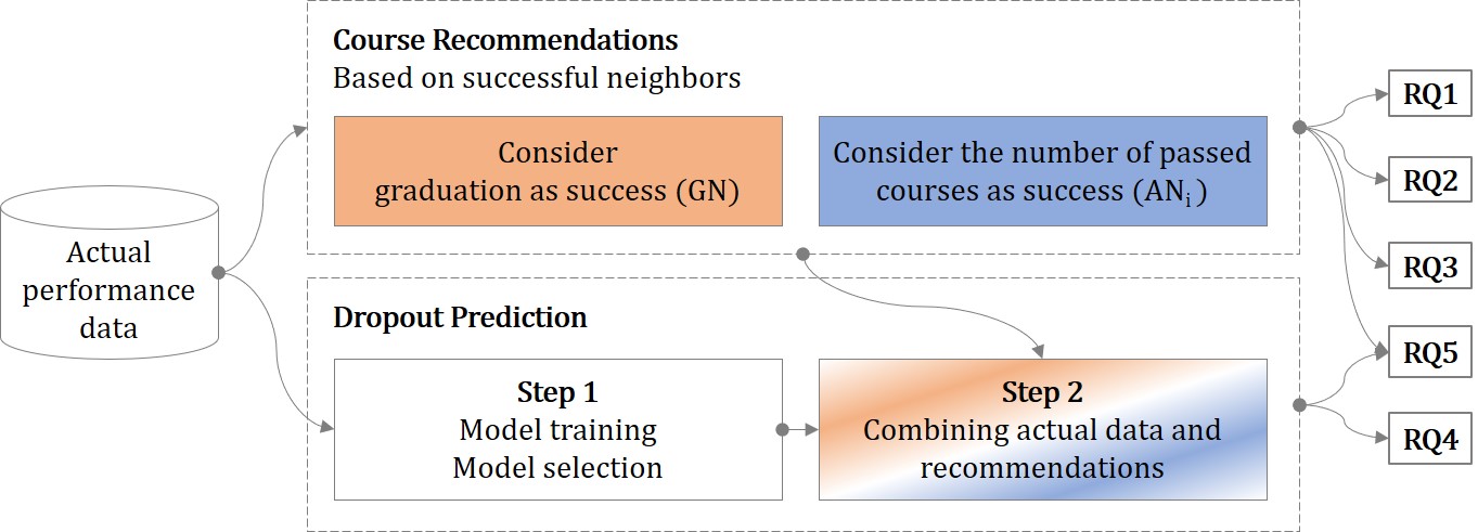
This section provides the representation of the data and the course recommender system that is based on success. It also outlines the general approach and the utilization of two types of successful students. The subsequent explanation covers the two-step dropout prediction process, including the training, optimization, and selection of models for the Step 1 Dropout Prediction, as well as the execution of the Step 2 Dropout Prediction. Figure 2 gives an overview of how the respective parts of the work are connected.
4.1. Data Representation
It is possible for a student to have multiple records for the same course in different semesters. For example, a student may enroll in a course in the first semester but not take the exam, then fail the exam in the next semester, and finally pass the exam in a following semester. In this case, a student has three different records for the same course in three different semesters. We assume that the entire history of a student’s academic performance is relevant, not just the final grade with which a course was passed. Therefore, we included the complete academic performance history and represented each student’s academic performance by a vector of grades.
Missing values. The algorithms used for course recommendations and dropout prediction require identical features, that is, grades in courses, for each semester and for all students. However, these algorithms cannot handle missing values, which can arise when students did not take the exam or did not enroll in a course. Therefore, we imputed the missing grades.
A. In terms of course recommendations and dropout prediction in Step 1. If students enrolled in a course but did not take the exam, a value of 6.0 was imputed; If they were not enrolled at all, a value of 7.0 was imputed. This means that not enrolling (7.0) is penalized more than enrolling but not taking the exam (6.0). The value of 6.0 aims to indicate that the students have engaged with the course, regardless of the specific duration of their participation. For example, they may have dropped out of the course some time during the semester, or they may have completed the course but did not take the exam, for example, due to insufficient preparation time.
B. In terms of the dropout prediction in Step 2. If we had an actual grade in the data records for that student and a recommended course, we used this grade. If we had no grade, we predicted a grade by imputation of the average of two medians: the median of all the grades that we know about from the student and the median of the historical grades for that course. This imputation rests on the strong assumption that underpins our recommendations as we explain in Section 4.2.1: the majority vote of the k-nearest neighbors yields a set of courses that a student can pass. We evaluated this prediction of grades using the actual known grades and obtained a Root Mean Square Error (RMSE, lower is better) of 0.634, which is comparable with RMSE scores from 0.63 to 0.73 to other studies in that field (Elbadrawy and Karypis, 2016, Polyzou and Karypis, 2016). For courses that were not recommended, we imputed a value of 7.0, following the same imputation method used when a student was not enrolled in any course, as in A.
Example. Table 1 illustrates the vector representation of six students for their first two semesters of study. Note that courses where all students have a grade of 7.0 are not shown. During the first semester, student 0 and their five neighbors passed all the courses in which they were enrolled with grades between 1.3 and 3.0. During the second semester, student 0 and neighbor #3 both did not pass course M11, receiving a grade of 5.0. Neighbor #5 did not take the exam of course M11 and a grade of 6.0 was imputed.
|
Semester
1
|
Semester
2
|
||||||||||||
|---|---|---|---|---|---|---|---|---|---|---|---|---|---|
| # | M01 | M02 | M03 | M04 | M05 | M08 | M09 | M10 | M11 | M12 | M13 |
Dist
|
|
| Student | 0 | 2.3 | 2.3 | 2.0 | 1.3 | 2.3 | 2.0 | 3.0 | 1.0 | 5.0 | 2.7 | 2.0 | |
| Neighbors | 1 | 2.0 | 2.0 | 2.0 | 1.3 | 3.0 | 1.7 | 3.0 | 1.0 | 4.0 | 2.7 | 2.3 | 1.4 |
| 2 | 2.0 | 2.7 | 2.0 | 1.7 | 2.7 | 1.3 | 3.0 | 1.3 | 4.0 | 2.7 | 1.7 | 1.5 | |
| 3 | 1.7 | 2.0 | 2.7 | 1.7 | 2.0 | 1.7 | 2.7 | 2.0 | 5.0 | 2.3 | 1.7 | 1.6 | |
| 4 | 2.0 | 2.7 | 2.0 | 2.0 | 2.7 | 2.0 | 3.0 | 1.3 | 3.7 | 3.0 | 2.0 | 1.7 | |
| 5 | 2.0 | 2.7 | 2.0 | 1.3 | 3.0 | 1.7 | 2.3 | 1.7 | 6.0 | 2.3 | 2.7 | 1.9 | |
| Color legend: | \(1.0\) | \(1.3\) | \(1.7\) | \(2.0\) | \(2.3\) | \(2.7\) | \(3.0\) | \(3.3\) | \(3.7\) | \(4.0\) | \(5.0\) | \(6.0\) | \(7.0\) |
4.2. Course Recommendations
4.2.1. Proposed Algorithm
The course recommender system is based on a KNN classifier and recommends courses to a student based on the courses passed by the student’s neighbors. The neighbors of a student are calculated once and, on their basis, the classification can be made for all courses: if the majority of the neighbors classify a course as passed for semester \(t+1\), it is recommended to the student for semester \(t+1\). Since we classified all courses passed by any neighbor of a student in semester \(t+1\), we got two sets for a student: recommended courses and not recommended courses. Given the possibility of recommending a course that the student has already passed, we removed those courses from the recommendation if present. We recommended courses for all 1,366 students to have the largest possible database to evaluate the recommendations.
Features. The features used to calculate the similarity between the students correspond to the features presented in Section 4.1. To generate course recommendations for the second semester, the neighbors were calculated based on the academic performance of their first semester, and the courses were recommended according to the majority of the neighbors in their second semester. Similarly, to generate the course recommendations for the third semester, the neighbors were calculated based on the academic performance of the first and second semesters, and the courses were recommended according to the majority of the neighbors in their 3rd semester.
Parameters. Two parameters have to be chosen for the nearest-neighbor algorithm: the metric to calculate the distance to neighbors and the number of neighbors \(k\). We selected the Euclidean distance as the distance metric for calculating the distances between the students since this is a well-known metric that should serve the understanding of the approach on the part of the students. The neighbors provide students samples of other students’ enrollment and passing experiences, which students look for when enrolling (Wagner et al., 2021). The course recommendations are affected by the number of neighbors, \(k\). We chose a value of \(k=5\) as it was considered suitable to reduce the risk of dropping out in Step 2 of the dropout prediction (Wagner et al., 2023). Building on our previous work and to reduce complexity, we limit our research in this paper again to \(k=5\) neighbors which matches the number of similar people used by Du et al. (2017) in their first series of user interviews.
Example. Table 2 presents the actual grades or imputed values for the courses in which the six students from Table 1 were enrolled during their third semester, the semester for which the course recommendation was generated in this example. To enable the comparison between student 0’s actual grades and the course recommendations, the actual grades for student 0 are shown (in italics). The recommended courses based on the nearest neighbor classification are M14, M15, M16, M18, and M19 (highlighted in blue). M14, for example, was recommended since the five neighbors passed M14 with grades between 1.7 and 3.0. M11 was not recommended since only neighbor #3 passed the course M11 with a grade of 2.7. However, student 0 actually passed M11 in semester 3 with a grade of 4.0. M17 was not recommended, as only two neighbors passed the course. Student 0 actually did not enroll in M17, so a 7.0 was imputed to represent the data point. M18 was recommended since four neighbors passed the course (#2 to #5). As student 0 was actually enrolled in M18 in semester 3 but did not take the exam, 6.0 was imputed.
|
Semester
3
|
||||||||
|---|---|---|---|---|---|---|---|---|
| # | M11 | M14 | M15 | M16 | M17 | M18 | M19 | |
| Student | 0 | 4.0 | 1.7 | 2.0 | 2.0 | 7.0 | 6.0 | 3.7 |
| Neighbors | 1 | 7.0 | 1.7 | 2.0 | 2.0 | 7.0 | 5.0 | 2.7 |
| 2 | 7.0 | 3.0 | 2.7 | 1.7 | 3.0 | 1.7 | 2.7 | |
| 3 | 2.7 | 2.0 | 2.0 | 7.0 | 7.0 | 2.0 | 3.3 | |
| 4 | 7.0 | 2.0 | 2.0 | 2.0 | 1.3 | 2.0 | 3.0 | |
| 5 | 7.0 | 1.7 | 1.7 | 2.0 | 7.0 | 2.7 | 3.7 | |
| Color legend: | \(1.0\) | \(1.3\) | \(1.7\) | \(2.0\) | \(2.3\) | \(2.7\) | \(3.0\) | \(3.3\) | \(3.7\) | \(4.0\) | \(5.0\) | \(6.0\) | \(7.0\) |
4.2.2. Risk Reducing Approach and Baseline
As already mentioned, we investigated two types of successful students: 1) graduated students GN and 2) all students ANi—graduated students and students who dropped out—with a minimum number of \(i\) passed courses in the semester. As a baseline for comparison, we used the data of all neighbors AN without a minimum number of courses passed as done in our previous work (Wagner et al., 2023). The study handbook indicates five or six courses, depending on the study program and the semester, as the number of courses that students should take in a semester.
We determined the largest minimum number of courses passed by calculating the number of potential neighbors. Table 3 illustrates that the inclusion of all neighbors (AN) or neighbors who have passed at least one to four courses ANi, \(1 \le i \le 4\), results in a larger pool of neighbors to select from compared to GN, which represents the pool of graduated students. The only exception to this is program AR in semester 3. Exceptions in terms of AN4 are program CM in semester 3 with the same number of students and program AR in semester 3 with a smaller number of students. By contrast, AN5 contains fewer students than GN for all programs and semesters, thus restricting not only the number, but perhaps also the diversity of the students included to generate the recommendations, which we think would be a too strong limitation. Therefore, we exclude this set of neighbors from our analysis.
In the following, we distinguish the subsequent neighbortypes: AN, AN1, AN2, AN3, AN4, and GN. AN and GN of the current work are identical to AN and GN of the approaches in our previous work; AN1, AN2, AN3, and AN4 are new to the present work. As mentioned in the introduction, using ANi for some \(i\) between 1 and 4 instead of GN would result in a recommender system that could reflect changes in the curriculum in a more timely manner.
| Minimum Number of Courses Passed
| ||||||||||
|---|---|---|---|---|---|---|---|---|---|---|
| Program | All (D+G) | D | G | S | 0 | 1 | 2 | 3 | 4 | 5 |
|
AR |
578 |
134 |
444 | 2 | 578 | 560 | 538 | 506 | 457 | 358 |
| 3 | 578 | 530 | 506 | 477 | 441 | 382 | ||||
|
CM |
527 |
221 |
306 | 2 | 527 | 454 | 414 | 382 | 328 | 258 |
| 3 | 527 | 403 | 375 | 346 | 306 | 235 | ||||
|
PT |
261 |
58 |
203 | 2 | 261 | 247 | 235 | 227 | 213 | 165 |
| 3 | 261 | 236 | 230 | 220 | 206 | 181 | ||||
4.3. Dropout Risk Prediction
The dropout prediction, a classification problem, was performed using the following two steps:
- Step 1:
- Models were trained, optimized, and evaluated using the actual enrollment and exam information to predict the two classes of the student status: dropout (D) or graduate (G).
- Step 2:
- We used the best model from Step 1 but replaced the data from the relevant semesters based on the course recommendations to predict dropout for the students in the test sets.
Our definition of dropout risk. The term dropout risk refers to the percentage of students in the test set who actually dropped out (as indicated in the Risk column of Table 4) or are predicted to drop out in Step 1 or Step 2. To determine whether the recommended courses help to reduce the dropout risk, we compare the predicted dropout risk P1 from Step 1 with the predicted dropout risk P2 from Step 2 (Table 9). The goal is for P2 to be less than P1.
4.3.1. Step 1 Dropout Prediction
For Step 1, models were trained and optimized using actual enrollment and exam information to predict the two classes of the student status: dropout (D) or graduate (G). The best models were selected for the prediction of the dropout in Step 1.
Feature set. Similarly to the course recommendations, the features we used to train the dropout prediction models in Step 1 correspond to the features presented in Section 4.1. The dropout prediction after the second semester was based on the academic performance of the first semester and the second semester, and the dropout prediction after the third semester was based on the academic performance of the first, second and third semesters. It is important to mention that our prediction did not focus on whether the students dropped out specifically after the first or second semester, but rather on whether they dropped out at some point or completed their studies.
| Student Status | Actual Dropout Risk
| |||||
|---|---|---|---|---|---|---|
| Program | Set | D | G | All (D+G) | Percentage | D/All
|
|
AR | Train | 91 | 371 | 462 | 19.7% | 91/462 |
| Test | 43 | 73 | 116 | 37.1% | 43/116 | |
|
CM | Train | 154 | 267 | 421 | 36.6% | 154/421 |
| Test | 67 | 39 | 106 | 63.2% | 67/106 | |
|
PT | Train | 37 | 171 | 208 | 17.8% | 37/208 |
| Test | 21 | 32 | 53 | 39.6% | 21/53 | |
| All | 413 | 953 | 1,366 | 30.2% | 413/1,366 | |
Train-test split. For dropout risk prediction, the data sets were sorted by the start of their study and split into 80% training data and 20% test data (Table 4), so the prediction evaluation was done based on students who started their studies last. The sorting is performed on the basis of the start date to reflect the real-world scenario. The students who have recently started their studies are the ones about whom we have the least information and these are the students for whom the predictions are specifically intended. Therefore, we used the data from these students to assess the effectiveness of the models. With this train-test split of the data, the dropout rate in the test data is typically higher than in the training data because it usually takes six semesters to know whether a student will graduate, whereas many students drop out of their studies much earlier. In addition, it is important to exclude currently active students to evaluate the prediction, as the final status of the students is needed. This exclusion had already taken place during the general data filtering, as explained in Section 3. As an example, the actual dropout risk of the program Architecture (AR), which represents the percentage of students who dropped out of the test set, is 0.371 (43 out of 116 students), as indicated in the Risk column of Table 4.
Model training. We trained models for each program (AR, CM, PT) and semesters \(t=2\) and \(t=3\). To detect a change in the dropout risk in Step 2, the models should be as accurate as possible, which we aimed to achieve through two approaches:
A. Training of different algorithms types. We trained the following algorithms in Python using scikit-learn (Pedregosa et al., 2011); settings that differ from the default are listed: decision tree (DT), LASSO (L, penalty=l1, solver=liblinear), logistic regression (LR, penalty=none, sol-ver=lbfgs), \(k\)-nearest neighbors (KNN), random forest (RF), and support vector machine with different kernels (SV: rbf, LSV: linear, PSV: poly).
B. Usage of different algorithm-independent approaches. Using our experience (Wagner et al., 2022), we kept the default hyperparameter settings of scikit-learn, except the settings to obtain a specific algorithm as mentioned above, in combination with the following list of algorithm-independent parameters.
- Feature selection by cut-off (CO):
We removed courses with too few grades and tried values between 1 and 5 as a minimum number of grades to retain a course; a value that is too high may result in the removal of recommended courses and thus would not be included in the dropout prediction. - Training data balancing (BAL):
We used two common techniques: RandomOverSampler (ROS) and Synthetic Minority Oversampling Technique (SMOTE) (Chawla et al., 2002), both implemented in imbalanced-learn, a Python library (Lemaître et al., 2017). - Decision threshold moving (DTM):
Usually, a classifier decides for the positive class at a probability greater than or equal to 0.5, but in the case of imbalanced data, it may be helpful to adjust this threshold, so, additionally to 0.5, we checked values between 0.3 and 0.6 in 0.05 steps. Lower and higher values did not lead to better results.
Model selection. To emphasize that both correct dropouts and correct graduates are important for prediction of dropout risk, we evaluated models based on test data using the Balanced Accuracy metric (BACC), defined as the mean of recall for class 1 (dropout), also known as true positive rate, and recall for class 0 (graduate), also known as true negative rate: \(BACC=(TP/P + TN/N)/2\) (higher is better).
Step 1 Dropout risk. Finally, we used the best models to predict the dropout risk for each program (AR, CM, PT) and semesters \(t=2\) and \(t=3\) for comparison with the Step 2 dropout risk.
4.3.2. Step 2 Dropout Prediction
To assess the impact of the course recommendations, the previously chosen models from Step 1 were again employed to predict the status of the students in the test set (dropout or graduation) by integrating the course recommendations.
Feature set and possible grade imputations. The dropout prediction for the second semester used the actual grades of the first semester and the recommendations for the second semester, while the dropout prediction for the third semester used the actual grades of the first and second semesters and the recommendations for the third semester. Since a course was recommended if the majority of neighbors passed that course, we could assume that the students were likely to pass the recommended courses.
Example. Consider again student 0 in Table 1 and Table 2 for the dropout predictions in Step 1 and Step 2. The grades and courses of the first and second semester were used for both steps and can be found in row 0 of Table 1. In addition to this, the actual grades from the third semester, that is, the courses M11, M14 to M16, and M19, were considered for the prediction in Step 1. These grades can be found in row 0 of Table 2. For the prediction in Step 2, the actual grades from the recommended courses M14 to M16, M18, and M19 were used. This means that the grade of 4.0 for M11 was replaced with 7.0, and the grade of 6.0 for M18 was replaced with the actual grade obtained by the student in a later semester or imputed as described previously.
5. RESULTS AND DISCUSSION
In this section, we present an in-depth analysis of the course recommendations regarding intersection (RQ1) and the number of courses (RQ2 and RQ3), as well as the dropout prediction models and the changes in dropout risk per neighbortype based on the two-step prediction (RQ4). Furthermore, we summarize the statistically significant differences between the neighbortype GN and the other neighbortypes ANi (RQ5).
5.1. RQ1: How large is the intersection between the set of courses recommended and the set of courses a student has passed?
5.1.1. RQ1 Evaluation
Since the course recommendations are for each course a binary classification problem, we employed a confusion matrix for each student (Table 5) to answer research question 1. We evaluated the recommendation for semester \(t+1\) for each student as follows: a course recommended and actually passed is a true positive (TP), a course recommended and actually not passed is a false positive (FP), a course not recommended but passed is a false negative (FN), and a course not recommended and not passed is a true negative (TN).
Metrics. To evaluate a set of recommended courses, it is important to measure both recall (whether passed courses include recommended courses) and precision (whether recommended courses include passed courses). We chose the F1 score to evaluate the intersections of the courses, as the F1 score represents both precision and recall. Furthermore, the F1 score ignores TN, which in our context is always a high value and therefore does not meet our needs. The score ranges from 0 to 1 with 1 indicating perfect classification (recall=1 and precision=1) and 0 indicating perfect misclassification (recall=0 or precision=0). The calculation is as follows: \(F1=2 \cdot TP / (2 \cdot TP + FP + FN)\).
In addition to the F1 score, we include recall as a commonly used metric for comparison with other studies (Ma et al., 2020, Polyzou et al., 2019). Recall represents the percentage of recommended courses based on the number of courses taken by student s. In our case, the recall is calculated as \(TP/P\).
It should be noted that there is a slight difference between our recall and recall\(@\)ns. Recall\(@\)ns may use the number of courses taken or enrolled in semester \(t+1\), whereas our definition considers the number of courses that were passed in semester \(t+1\). This distinction is important because our aim is to recommend courses with a high probability of passing. Hence, our assessment is more stringent. Another type of recall, recall\(@\)n (Elbadrawy and Karypis, 2016, Pardos et al., 2019), fixes the number of recommended courses at n. However, it is not applicable in our case since we do not rank the recommendations and may suggest more or fewer than \(n\) courses.
| Predicted positive | Predicted negative | Totals | |
|
Actual positive | Passed and recommended True positive TP | Passed but not recommended False negative FN | Passed P |
|
Actual negative | Not passed but recommended False positive FP | Not passed and not recommended True negative TN | Not passed |
| Totals | Recommended | Not recommended | All courses |
| F1 | |||||||
|---|---|---|---|---|---|---|---|
| ST | PS | AN | AN1 | AN2 | AN3 | AN4 | GN |
|
D | AR2 | 0.481 | 0.514 | 0.528 | 0.529 | 0.534 | 0.521 |
| AR3 | 0.279 | 0.313 | 0.345 | 0.342 | 0.332 | 0.305 | |
| CM2 | 0.328 | 0.384 | 0.414 | 0.421 | 0.419 | 0.397 | |
| CM3 | 0.130 | 0.156 | 0.168 | 0.175 | 0.179 | 0.159 | |
| PT2 | 0.511 | 0.545 | 0.536 | 0.514 | 0.505 | 0.528 | |
| PT3 | 0.112 | 0.141 | 0.150 | 0.152 | 0.151 | 0.156 | |
|
G | AR2 | 0.854 | 0.862 | 0.867 | 0.870 | 0.878 | 0.871 |
| AR3 | 0.817 | 0.830 | 0.839 | 0.848 | 0.853 | 0.842 | |
| CM2 | 0.824 | 0.839 | 0.848 | 0.856 | 0.865 | 0.851 | |
| CM3 | 0.711 | 0.735 | 0.746 | 0.758 | 0.771 | 0.755 | |
| PT2 | 0.837 | 0.832 | 0.835 | 0.835 | 0.836 | 0.828 | |
| PT3 | 0.335 | 0.343 | 0.346 | 0.347 | 0.345 | 0.356 | |
| All | 0.618 | 0.637 | 0.648 | 0.653 | 0.657 | 0.646 | |
| Recall
| |||||||
| ST | PS | AN | AN1 | AN2 | AN3 | AN4 | GN |
|
D | AR2 | 0.553 | 0.607 | 0.645 | 0.658 | 0.694 | 0.649 |
| AR3 | 0.345 | 0.389 | 0.445 | 0.461 | 0.473 | 0.417 | |
| CM2 | 0.383 | 0.450 | 0.513 | 0.553 | 0.570 | 0.498 | |
| CM3 | 0.141 | 0.171 | 0.192 | 0.206 | 0.221 | 0.187 | |
| PT2 | 0.577 | 0.616 | 0.648 | 0.656 | 0.656 | 0.651 | |
| PT3 | 0.113 | 0.137 | 0.144 | 0.155 | 0.161 | 0.140 | |
|
G | AR2 | 0.896 | 0.904 | 0.913 | 0.922 | 0.942 | 0.925 |
| AR3 | 0.835 | 0.851 | 0.864 | 0.879 | 0.892 | 0.875 | |
| CM2 | 0.851 | 0.870 | 0.882 | 0.900 | 0.921 | 0.895 | |
| CM3 | 0.727 | 0.762 | 0.776 | 0.796 | 0.814 | 0.788 | |
| PT2 | 0.834 | 0.836 | 0.842 | 0.844 | 0.851 | 0.844 | |
| PT3 | 0.261 | 0.270 | 0.273 | 0.277 | 0.278 | 0.284 | |
| All | 0.641 | 0.665 | 0.684 | 0.699 | 0.715 | 0.689 | |
| Color legend: | \(<0.2\) | \(<0.3\) | \(<0.4\) | \(<0.5\) | \(<0.6\) | \(<0.7\) | \(<0.8\) | \(<0.9\) | \(<1.0\) |
Aggregation for groups of students. We evaluated how the set of recommended courses intersects with the set of courses that students have passed using the means of individual F1 and recall scores. To better distinguish for which student groups the recommendations better align with actual courses passed, the scores are grouped by student status ST (D: dropouts, G: graduates), program and semester PS (AR2 to PT3), and neighbortypes (AN, AN1, AN2, AN3, AN4, and GN). The results are given in Table 6.
5.1.2. RQ1 Example
Scores for a single student. Looking at the recommendations for student 0 in Table 2, the courses M14 to M16 and M19 were passed and recommended (TP), M11 was passed but not recommended (FN), M17 was not passed and not recommended (TN), M18 was not passed but recommended (FP), and all the other courses not shown here are also not passed and not recommended (TN). Therefore, we can calculate \(F1=2 \cdot 4 / (2 \cdot 4 + 1 + 1)= 0.8\) and \(Recall=4/5=0.8\).
Scores for a group of students. Taking students who dropped out of the CM study program and their course recommendations for semester 2 as an example (see row "D > CM2" in the upper portion of Table 6), we get an F1 score of 0.328 for recommendations based on all neighbors (AN), 0.421 for recommendations based on students who passed at least three courses (AN3), and 0.397 for recommendations based on neighbors who graduated (GN).
Looking at students from progam CM who graduated (G) and their course recommendations for semester 2 (see row "G > CM2" in the upper portion of Table 6), the F1 score is much higher: 0.824 for recommendations calculated with AN, 0.856 for recommendations calculated with AN3, and 0.851 for recommendations calculated with GN.
Recall, again for students from program CM and their recommendations for semester 2 (see rows "D > CM2" and "G > CM2" in the lower portion of Table 6), is 0.553 for students with status D when recommendations are calculated with AN3, and 0.900 – again much higher – for students with status G calculated with AN3.
5.1.3. RQ1 Findings and Discussion
We look at the question "How large is the intersection between the set of courses recommended and the set of courses a student has passed?" from two perspectives: "graduates and dropouts" and "second and third semester."
Graduates and dropouts. The recommendations should show another, more promising way of studying to students who are struggling while they should not disturb students who are doing well. Thus, we expect the F1 score and recall to be much higher for students with status G than for students with status D. As expected, the mean F1 score and recall are always higher for students with status G than for students with status D across all types of successful students. Although F1 tends to be around 0.5 for students with status D, it is near 0.8 or higher for students with status G, especially when considering the neighbors of the sets AN3, AN4, or GN. A similar pattern can be observed for recall. This means that the recommended courses reflect quite well how these students study. An exception is program PT and semester 3. This might be due to the high number of elective courses offered by that program in semester 3. Of the 26 courses recommended to at least one student and also used in dropout prediction, only one is mandatory; the other 25 are electives. In addition, the number of students is lower than in the other two study programs.
Second and third semester. The mean F1 score and the mean recall are higher in all cases for the second semester than for the third semester. The higher the semesters, the more the sets of courses which students pass drift apart. On the one hand, this makes it more difficult to find close neighbors, and on the other hand, it makes the recommendation itself more difficult: the neighbors sometimes disagree and have passed too many different courses, which means that no majority can be found for many courses and these courses are not recommended. This is particularly true for PT3 due to the high number of elective courses, as already mentioned.
Summary. Overall, the results indicate that the recommended courses match the courses passed by students who graduated quite well and show another way of studying to students who dropped out. The results also confirm a limitation of the proposed recommendations when the study degree program foresees many elective courses in a semester.
For comparison with related work, we provide the mean F1 score for all students across programs and semesters for all neighbortypes (see row "All" at the bottom of Table 6): AN4 achieves the highest mean F1 score with a value of 0.657 and also the highest mean recall with a value of 0.715. The scores of Ma et al. (2020) varied between 0.431 and 0.472, depending on the semester. Polyzou et al. (2019) achieved an average score of 0.466.
5.2. RQ2: How many courses are recommended?
5.2.1. RQ2 Evaluation
To answer research question 2, we first look at the number of courses recommended for the semester \(t+1\). Using box plots, we visualize the distribution of students by the number of recommended courses (Figure 3). To explore why some students received no or only a few recommendations, we describe the relationship between the number of recommended courses and the distance between students and their neighbors using a scatter plot (Figure 4).
Number of recommended courses. Figure 3 presents the number of recommended courses per study program and semester PS (AR2 to PT3), and student status (D: dropouts, G: graduates) as five-number summary in the form of box plots. The neighbortypes (AN to GN) are represented by different colors. In each study program and semester, the box plots on the left concern students with status D while the ones on the right concern students with status G. Looking at the leftmost box plot in each case shows that calculating the recommendations with the set AN can lead to empty recommendations (0 course recommended), especially for students with status D. For exact quartiles and medians, see Table 11 in the appendix.
Investigation of the small number of courses recommended. The scatterplots in Figure 4 illustrate the mean distance in the CM program between students and their neighbors in relation to the number of recommended courses. The scatterplots are separated by semester (CM2 on the left, CM3 on the right) and neighbortype (AN to GN), with each student’s status (D: dropouts, G: graduates) represented by different colors. In addition, the underlying bar chart displays the number of students for each number of courses. See also Figure 5 in the Appendix, which gives the plots for the two other study programs. For the exact numbers of students and mean distances, see Table 12 for dropouts and Table 13 for graduates.
5.2.2. RQ2 Example
Number of recommended courses. The middle row left in Figure 3, CM2, shows the quartiles and outliers of the number of recommended courses for the program CM and semester 2 per type of neighbor. The 25% percentile of AN2, AN3, AN4, and GN for students with status G is 5; the median and 75% percentile are merged everywhere at the value 6. This means that most of these students get five or six recommended courses. Some outliers get one, two, or three courses recommended. In contrast, most of the students with status D get between three and five courses recommended when the recommendations are calculated with sets AN2, AN3, or GN: these students tend to get fewer courses recommended than the students with status G.

Investigation of the small number of courses recommended. On the upper left of Figure 4 in the second semester with neighbortype AN, title CM2 AN, 90 students get 0 courses recommended; the average distance between students with status D from their neighbors is about 2, while it is about 3.5 for students with status G. When comparing the second and third semesters for program CM and neighbor AN, still for 0 recommended courses, it can be observed that the mean distances are higher for the third semester compared to the second semester. This trend holds for students who dropped out and for students who graduated. By examining the background bars, only for the first row of scatter plots in this example (CM2 - AN and CM3 - AN), it can be observed that a higher number of students did not receive course recommendations for the third semester compared to the second semester.

5.2.3. RQ2 Findings and Discussion
The percentage of students who receive no recommendation or only one recommended course is much smaller when the recommendations are calculated with any type of neighbors except AN and to some extent AN1. This is especially noticeable for students who dropped out. The box plots calculated with AN1 to AN4 do not differ much from the box plot calculated with GN for students with status G. This is not true for students with status D; the box plots calculated with AN2 or AN3 tend to be more similar to the box plot calculated with GN than the box plots calculated with the other sets. For graduates in AR, CM, and PT programs in semester 2, the number of recommended courses for the majority of students is close to the number planned in the curriculum, that is, five or six courses. Again, PT - semester 3 differs. As is visible in the evaluation of the intersection in Section 5.1, there is less agreement about the courses among the neighbors, which can be explained by a large number of elective courses in semester 3. This leads to smaller set sizes for course recommendations. Our results also show that students who are very different from their neighbors, especially those with status G, are likely to receive few recommendations.
5.3. RQ3: Does the number of courses recommended differ from the number of courses passed and enrolled in by students?
5.3.1. RQ3 Evaluation
To answer research question 3, we calculated the median differences between the number of recommended courses and the number of courses enrolled (R - E), and the median difference between the number of courses recommended and the number of courses passed (R - P) (Table 7). To better distinguish for which student groups the recommendations are closer to the actual numbers, the results are grouped by student status (D: dropout, G: graduates), neighbortypes (AN to GN), program, and semester.
5.3.2. RQ3 Example
We consider study program CM and semester 2. The left part of Table 7, R - E, shows the median difference between the number of recommended courses and the number of courses that students enrolled in. We consider first students who dropped out (D). The columns AN2, AN3, AN4, and GN have all the value -1.0 for CM2, which means that the number of recommended courses is on average 1 less than the number of courses the students enrolled in. Comparing the number of recommended courses with the number of those passed, R - P, the right part of Table 7, we see a value of 2.0 for the types AN2, AN3, and GN, meaning that the number of recommended courses is on average 2 more than the number of courses passed by students. Considering students who graduated, we see no difference in the number of courses recommended, enrolled in, and passed on average: all values are 0.
| R - E | R - P
| ||||||||||||
| ST | PS | AN | AN1 | AN2 | AN3 | AN4 | GN | AN | AN1 | AN2 | AN3 | AN4 | GN |
|
D | AR2 | -2.0 | -1.0 | -1.0 | -1.0 | 0.0 | -1.0 | 0.5 | 1.0 | 1.0 | 2.0 | 2.0 | 1.0 |
| AR3 | -3.0 | -2.0 | -1.0 | -1.0 | 0.0 | -1.0 | 0.0 | 1.0 | 2.0 | 3.0 | 3.0 | 2.0 | |
| CM2 | -3.0 | -2.0 | -1.0 | -1.0 | -1.0 | -1.0 | 0.0 | 1.0 | 2.0 | 2.0 | 3.0 | 2.0 | |
| CM3 | -4.0 | -3.0 | -2.0 | -2.0 | -1.0 | -2.0 | 0.0 | 0.0 | 1.0 | 1.0 | 2.0 | 1.0 | |
| PT2 | -2.0 | -2.0 | -1.0 | -1.0 | -1.0 | -1.0 | 1.0 | 1.0 | 1.0 | 2.0 | 2.0 | 1.0 | |
| PT3 | -5.0 | -4.0 | -4.0 | -4.0 | -3.0 | -4.0 | -0.5 | 0.0 | 0.0 | 0.0 | 0.0 | 0.0 | |
|
G | AR2 | 0.0 | 0.0 | 0.0 | 0.0 | 0.0 | 0.0 | 0.0 | 0.0 | 0.0 | 0.0 | 0.0 | 0.0 |
| AR3 | 0.0 | 0.0 | 0.0 | 0.0 | 0.0 | 0.0 | 0.0 | 0.0 | 0.0 | 0.0 | 0.0 | 0.0 | |
| CM2 | 0.0 | 0.0 | 0.0 | 0.0 | 0.0 | 0.0 | 0.0 | 0.0 | 0.0 | 0.0 | 0.0 | 0.0 | |
| CM3 | -1.0 | 0.0 | 0.0 | 0.0 | 0.0 | 0.0 | 0.0 | 0.0 | 0.0 | 0.0 | 0.0 | 0.0 | |
| PT2 | 0.0 | 0.0 | 0.0 | 0.0 | 0.0 | 0.0 | 0.0 | 0.0 | 0.0 | 0.0 | 0.0 | 0.0 | |
| PT3 | -4.0 | -4.0 | -4.0 | -3.0 | -3.0 | -3.0 | -3.0 | -3.0 | -3.0 | -3.0 | -3.0 | -3.0 | |
5.3.3. RQ3 Findings and Discussion
On the one hand, the recommender system suggests to students who dropped out to focus on fewer courses; all columns of the left part R - E have negative values except for the column AN4. In contrast, the columns of the right part R - P have almost everywhere positive values, that is, students should enroll in fewer courses with the expectation that they can pass more courses instead, except in PT3. On the other hand, nothing changes on average for graduates: There is no difference, except for PT3 again. The problem with PT3 is the lower number of recommended courses in general, as also visible in Figure 3, which can be explained by a large number of elective courses, as already written.
5.4. RQ4: Do the recommendations lower the risk of dropping out?
5.4.1. RQ4 Evaluation
To answer research question 4, we compare the dropout risk, that is, the proportion of students who are predicted to drop out P2, based on the predictions from Step 2 with the dropout risk P1 from Step 1.
Step 1. We selected the models—trained with actual exam and enrollment data—with the highest BACC for each program and semester (Table 8). They differ in terms of their algorithm-independent parameters. We obtain P1 as the Step 1 dropout risk, that is, the proportion of students in the test set predicted to drop out, which we compare later with the Step 2 dropout risk P2.
Step 2. Using again the best models from Step 1, we performed the Step 2 prediction using the recommendations. Table 9 shows the difference between the dropout risk P2 from Step 2 and P1 from Step 1 for each neighbortype (AN to GN). We distinguish the predicted dropout risk by student status (D: dropouts, G: graduates) for a better overview of how the models perform.
| Model Characteristics | |||||||
| PS | C | CO/F | DTM | BAL | BACC | REC | P1 |
| AR2 | RF | 0/38 | 0.35 | SMOTE | 0.866 | 0.814 | 0.353 |
| AR3 | RF | 4/32 | 0.45 | ROS | 0.935 | 0.884 | 0.336 |
| CM2 | SV | 1/36 | 0.30 | None | 0.920 | 0.866 | 0.557 |
| CM3 | RF | 0/74 | 0.45 | SMOTE | 0.927 | 0.881 | 0.566 |
| PT2 | LSV | 3/16 | 0.30 | SMOTE | 0.913 | 0.857 | 0.358 |
| PT3 | LSV | 3/47 | 0.30 | SMOTE | 0.882 | 0.857 | 0.396 |
5.4.2. RQ4 Example
Regarding Step 1. Table 8 provides information on the best classifiers. Consider the study program CM and semester 2. The support vector (SV) classifier (column C) achieved the best BACC when removing all courses that do not have at least one grade (column CO) resulting in 36 features (column F), representing 36 courses; the decision threshold (column DTM) is 0.3, which means that students are predicted to drop out already at a 30% probability; the training set was not balanced (column BAL). Compared to the actual risk of dropping out as the percentage of students who dropped out of the test data, 0.632 (Table 4, row "CM > Test"), the predicted risk in Step 1 is lower (P1=0.557).
Regarding Step 2. Considering CM2 again in Table 9: the dropout risk of Step 2 of students who actually dropped out (D) is 9.0% lower using AN and 14.9% lower using AN3 or GN than in Step 1. Looking at students who actually graduated (G), the dropout risk for Step 2 is 2.6% higher than in Step 1. Thus, if we use the course recommendations and assume that these exact courses are passed, the risk decreases by at least 9.0% for actual dropouts and increases by 2.6% for actual graduates. Based on the size of the test dataset (Table 4), this implies the following in absolute numbers: out of the 67 students who dropped out, 6 more students are predicted to graduate and of the 39 students who graduated, one more student is predicted to drop out in Step 2 compared to the prediction in Step 1.
| ST | PS |
AN
|
AN1
|
AN2
|
AN3
|
AN4
|
GN
|
|---|---|---|---|---|---|---|---|
|
D | AR2 | -0.140 | -0.140 | -0.140 | -0.209 | -0.233 | -0.256 |
| AR3 | -0.163 | -0.233 | -0.419 | -0.535 | -0.628 | -0.605 | |
| CM2 | -0.090 | -0.104 | -0.104 | -0.149 | -0.209 | -0.149 | |
| CM3 | -0.060 | -0.090 | -0.149 | -0.179 | -0.194 | -0.164 | |
| PT2 | -0.238 | -0.238 | -0.238 | -0.238 | -0.286 | -0.238 | |
| PT3 | 0.048 | 0.048 | 0.048 | 0.000 | 0.000 | -0.048 | |
|
G | AR2 | -0.068 | -0.068 | -0.068 | -0.068 | -0.055 | -0.055 |
| AR3 | 0.027 | 0.014 | 0.000 | -0.014 | -0.014 | -0.014 | |
| CM2 | 0.026 | 0.026 | 0.026 | 0.026 | 0.026 | 0.026 | |
| CM3 | 0.026 | 0.026 | 0.026 | 0.000 | 0.000 | 0.000 | |
| PT2 | 0.375 | 0.344 | 0.344 | 0.344 | 0.281 | 0.281 | |
| PT3 | 0.156 | 0.156 | 0.156 | 0.125 | 0.125 | 0.094 | |
| All | -0.008 | -0.022 | -0.043 | -0.075 | -0.099 | -0.094 |
| Color legend: | \(<-0.6\) | \(<-0.5\) | \(<-0.4\) | \(<-0.3\) | \(<-0.2\) | \(<-0.1\) | \(<0.0\) | \(<0.1\) | \(<0.2\) | \(<0.3\) | \(<0.4\) |
5.4.3. RQ4 Findings and Discussion
Step 1. The best models have been obtained when the training data were balanced except for program CM and semester 2. The predicted dropout risk P1 is lower in all cases than the actual dropout risk, see column Risk for the test set in Table 4, as we have observed for CM2, except for PT3 where it is equal. This means that our models tend to be optimistic and predict as graduates some students who dropped out. The general accuracy of the prediction in Step 1 should be further optimized.
Step 2. We further look at the question "Do the recommendations lower the risk of dropping out?" from two perspectives: "graduates and dropouts" and "second and third semester."
Graduates and dropouts. As we analyze Table 9, we expect the values to be equal to or less than 0, and this is true for students with status D, who are the primary focus of our recommendations. For status D, except for the study program PT, we observe that the values of columns AN3 and AN4 are closer to the values of column GN than AN. This is less true for columns AN1 and AN2. For students with status G, the values are much smaller than for students with status D, which we expect. These students have graduated and the recommendations should not really change the outcome for them. However, for the program CM semester 2 and the program PT, the values are higher than 0, specifically for status G. A glance at Table 4 reveals that the number of students with status G is small in the test set of CM2, while the program PT has a smaller number of students overall than the other two programs. This could explain these somewhat negative results, particularly for the PT program and the subgroup with status G.
Second and third semester. We do not expect large differences between the values for the second and third semesters, regardless of study program, status, and type of successful students. However, we see that the values in row AR3 are noticeably lower than the values in row AR2 for students with status D. This is probably due to the fact that on average more courses are recommended for students with status D in AR3 than in CM3 and PT3, see Figure 3. Furthermore, the PT program is an exception, and the results, especially for status G, are not as expected. We conjecture that this is primarily based on the small number of students enrolled in that program, see Table 4, and secondarily, on the high number of elective courses proposed in semester 3 of this study program. As students can freely choose five courses from six among a list of about 25 courses, it is more difficult for the algorithm to calculate accurate recommendations.
5.5. RQ5: Do the different approaches to define successful students give statistically significant different recommendations results?
5.5.1. RQ5 Evaluation
To address research question 5, we performed significance tests for subpopulations using a significance level of 0.05. These subpopulations were defined based on the program (AR, CM, PT), semester (2, 3), and student status (D, G). For example, a subpopulation were students in AR2 who dropped out. Our aim was to detect any statistically significant differences between the recommendation approach \(GN\) and all other approaches AN to AN4 in relation to three specific aspects:
- (i)
- the predicted dropout probability in Step 2 (P2),
- (ii)
- the intersection of courses recommended and courses actually passed (F1)
- (iii)
- the number of recommended courses (R),
Overall, we had 36 cases for each neighbortype: 3 study programs \(\times \) 2 semesters \(\times \) 2 student statuses \(\times \) 3 aspects.
Test choice. As visible in the histograms and confirmed by the Kolmogorov-Smirnov test, the data tested are not normally distributed. Consequently, we used the Wilcoxon signed-rank test to assess the statistical differences between the GN approach and the other approaches. Approaches relevant to the present work are those that do not indicate statistically significant differences, i.e., with a significance >=0.05. This would suggest that the differences between the approaches are random, and thus provide similar recommendations. All tests were performed in Python using SciPy (Virtanen et al., 2020).
Table 10 provides the number of cases for each aspect (P2, F1, R) and student status (D: dropouts, G: graduates) with a maximum of 6 cases (3 study programs \(\times \) 2 semesters) in which the difference was not statistically significant. The row "All" gives the sum of the cases for each neighbortype (AN to AN4) out of 36. Table 14 in the appendix provides the exact p-values for each case.
Multiple statistical testing. We are aware that with an increasing number of statistical tests, the risk of false finding of statistical significance increases. However, in our particular case, it is not our objective to identify statistically significant differences. Rather, our objective is to identify and highlight the absence of statistically significant differences. As a result, we have chosen not to adjust the p-values.
5.5.2. RQ5 Example
When analyzing the data in Table 10 for F1 and the students who dropped out (row "F1 > D"), it becomes apparent that the course recommendations based on all students (AN) are not significantly different from the course recommendations based on students who graduated (GN) in half of the cases (3 out of 6). However, when the minimum number of courses passed increases to 1 (neighbortype AN1), the course recommendations no longer show statistically significant differences in the six possible cases (programs and semesters, AR2 to PT3). However, increasing the minimum number of courses passed further leads to the reemergence of statistically significant differences. The number of cases is generally smaller when examining students who dropped out based on F1, but remains high for neighbortype AN2 and neighbortype AN3 and even higher for these two neighbor types compared to students who dropped out.
|
Aspect
|
ST
|
AN | AN1 | AN2 | AN3 | AN4 |
|---|---|---|---|---|---|---|
|
P2 | D | 1 | 2 | 2 | 3 | 2 |
| G | 3 | 4 | 4 | 6 | 6 | |
|
F1 | D | 3 | 6 | 5 | 4 | 4 |
| G | 1 | 2 | 6 | 5 | 2 | |
|
R | D | 0 | 1 | 3 | 3 | 0 |
| G | 0 | 0 | 0 | 5 | 2 | |
| All | 8 | 15 | 20 | 26 | 16 | |
5.5.3. RQ5 Findings and Discussion
It turns out that AN3 is most often not statistically significant different from GN (26 out of 36 cases), followed by AN2 (20 cases) and AN4 (16 cases). This indicates that the differences in the considered aspects and subpopulations are probably random. This is especially valid for students who have graduated (status G), as AN3 can be considered equivalent to GN in 16 of 18 cases (3 study programs \(\times \) 2 semesters \(\times \) 1 student status \(\times \) 3 aspects), see Table 14. It should also be noted that AN3 and GN do not differ statistically significantly in a consistent manner. For example, looking at AR2 and status D, the tests for P2 and R indicate a statistically significant difference, but not the test for F1. These results suggest that AN3 provides an alternative to GN, which, on the one hand, is equally based on success and, on the other hand, supports the faster growth of the database for course recommendations and the ability to react more quickly to changes in the curriculum.
6. CONCLUSION, LIMITATIONS, AND FUTURE WORK
This paper presents a comprehensive evaluation of a novel course recommender system designed to primarily support students who face difficulties in their initial semesters and are at risk of dropping out. The evaluation uses data from three distinct study programs that vary in terms of subject matter, student population, and program structure, including a program with a high number of elective courses in the third semester.
The evaluation shows that considering students who passed at least three courses in a semester (AN3) to calculate the recommendations is a viable alternative to considering students who graduated (GN), as was done in our previous work (Wagner et al., 2023). Indeed, the results of the different evaluations obtained in the present work show that the number of recommended courses when calculated with AN3 is similar to the number of recommended courses when calculated with GN. The F1 and recall scores tend to be slightly higher when calculated with AN3 while the changes in the dropout risk tend to be slightly higher when calculated with GN. Furthermore, the significance tests show that in most cases, the differences are not statistically significant. As already mentioned, a practical relevance in opting for AN3 is that student data could be used earlier and, thus, changes in the curriculum could be taken into account in a more timely manner. Interestingly, three is half of the number of courses students should take according to the study handbook.
The evaluation of the first research question reveals that the recommended courses generally align with the courses passed by the students who have graduated. However, there is an exception in the third semester of the PT program, which offers many elective courses, resulting in fewer alignments. The situation differs for students who dropped out as the recommended courses are less consistent with the courses they have passed. The recommendations suggest a different approach to study.
The evaluations of the second and third research questions indicate that the number of recommended courses for students who graduate is close to the number of courses planned in the curriculum, except for the aforementioned third semester of program PT. However, for students who dropped out, the number of recommended courses is generally lower than the number of courses in which they were enrolled, suggesting that it might be beneficial for them to focus on a smaller number of courses, as suggested by the recommendations.
For the evaluation of the fourth research question, we assumed that all students would successfully complete the recommended courses. The findings suggest that these recommendations lead to a reduction in the risk of dropping out, particularly for the targeted at-risk students who dropped out. However, the results are less conclusive for students who graduated, possibly due to limited data available for analysis in the test set.
The evaluation of the fifth research question indicates that AN3 can be considered as equivalent to our previous success-based approach in almost all aspects explored for the students who graduated. It can also be seen as a viable alternative to GN for all students.
In summary, the paths followed by successful students are helpful to other students, especially those who struggle. It is worth noting that our course recommendation approach is generalizable even when enrollment data are not available, that is, when students have enrolled in a course but did not take the exam, which is the case in certain institutions. With the exception of addressing missing values and comparing the number of recommended courses with the number of enrolled courses, as investigated in our third research question, the evaluation process remains the same.
Limitations. The evaluations have identified two main limitations in our recommender system. Firstly, it is more suitable for curricula that consist primarily of mandatory courses that all students must pass, which is often the case in the first two semesters of a program. This is also the period in which student dropout is the most frequent. Secondly, the system recommends very few courses for students who have distant neighbors. Therefore, it is necessary to explore a different approach to handling the courses passed in the recommender system. Additionally, the results indicate that the use of machine learning algorithms for evaluation purposes may have limitations in situations with a small student population, specifically in our case for study program PT. Although there is a potential drawback to offering recommendations that may be inaccurate or unhelpful, the recommender system enables us to showcase the academic paths of five students who have similar performance as a stimulus. Any tool built on our prototype should present these recommendations to students as suggestions, ensuring that they understand the reasoning behind the suggestions and giving them the autonomy to decide whether or not to follow them.
Future work. A preliminary evaluation with students indicated that the recommendations are understandable (Wagner et al., 2023). Building on our work on the recommendation system, we conducted in parallel to this study a survey with students to assess the explainability and quality of the recommendations (Wagner et al., 2024). In addition to the course recommendations as sets, the recommendations were extended to take the form of ranked lists. For example, consider Student 0 and Table 2. The ranked list of courses (M14, M15, M19, M16, M18, M17, M11) based on the number of students who passed the courses would then be compared with the set {M14, M15, M16, M18, M19}. The results showed that the students generally trust and understand the recommender system, with no general significant preference for the rank list or the set.
Investigating the benefits and drawbacks of using sets instead of ranked lists is a future work. Furthermore, it is necessary to evaluate what additional support students need to pass all recommended courses, aside from taking fewer and different courses than they might think. As another direction for future work, we consider the inclusion of data from currently enrolled students. This would enable a broader range of potential nearest neighbors, potentially yielding different outcomes. An analysis of fairness, in our case due to the data situation for gender, should still be carried out.
DECLARATION OF GENERATIVE AI SOFTWARE TOOLS IN THE WRITING PROCESS
During the preparation of this work, the authors used https://www.deepl.com/, https://quillbot.com/, and https://www.writefull.com/in all sections to achieve better translations and more fluent texts. After using these services, the authors reviewed and edited the content as needed and take full responsibility for the content of the publication.
EDITORIAL STATEMENT
Agathe Merceron had no involvement with the journal’s handling of this article in order to avoid a conflict with her Editor role. The entire review process was managed by Special Guest Editors Mingyu Feng and Tanja Käser.
REFERENCES
- Aulck, L., Nambi, D., Velagapudi, N., Blumenstock, J., and West, J. 2019. Mining University Registrar Records to Predict First-Year Undergraduate Attrition. In Proceedings of the 12th International Conference on Educational Data Mining (EDM 2019), C. F. Lynch, A. Merceron, M. Desmarais, and R. Nkambou, Eds. International Educational Data Mining Society, Montreal, Canada, 9–18. https://eric.ed.gov/?id=ED599235.
- Berens, J., Schneider, K., Gortz, S., Oster, S., and Burghoff, J. 2019. Early Detection of Students at Risk - Predicting Student Dropouts Using Administrative Student Data from German Universities and Machine Learning Methods. Journal of Educational Data Mining 11, 3, 1–41. https://doi.org/10.5281/zenodo.3594771.
- Chawla, N. V., Bowyer, K. W., Hall, L. O., and Kegelmeyer, W. P. 2002. SMOTE: Synthetic Minority Over-sampling Technique. Journal of Artificial Intelligence Research 16, 321–357. http://arxiv.org/abs/1106.1813.
- Du, F., Plaisant, C., Spring, N., and Shneiderman, B. 2017. Finding Similar People to Guide Life Choices: Challenge, Design, and Evaluation. In Proceedings of the 2017 Conference on Human Factors in Computing Systems (CHI 2017). Association for Computing Machinery, New York, NY, USA, 5498–5544. https://doi.org/10.1145/3025453.3025777.
- Elbadrawy, A. and Karypis, G. 2016. Domain-Aware Grade Prediction and Top-n Course Recommendation. In Proceedings of the 10th ACM Conference on Recommender Systems (RecSys 2016). Association for Computing Machinery, New York, NY, USA, 183–190. https://doi.org/10.1145/2959100.2959133.
- Heublein, U., Ebert, J., Hutzsch, C., Isleib, S., König, R., Richter, J., and Woisch, A. 2017. Zwischen Studienerwartungen und Studienwirklichkeit. Ursachen des Studienabbruchs, beruflicher Verbleib der Studienabbrecherinnen und Studienabbrecher und die Entwicklung der Studienabbruchquote an deutschen Hochschulen. [Between study expectations and study reality. Causes of dropping out of university, where dropouts remain in their careers and the development of the dropout rate at German universities.]. Collection, Deutsches Zentrum für Hochschul- und Wissenschaftsforschung (DZHW). June. https://www.bildungsserver.de/onlineressource.html?onlineressourcen_id=58641.
- Heublein, U., Hutzsch, C., and Schmelzer, R. 2022. Die Entwicklung der Studienabbruchquoten in Deutschland [The development of student drop-out rates in Germany]. Tech. rep., Deutsches Zentrum für Hochschul- und Wissenschaftsforschung (DZHW). https://www.dzhw.eu/publikationen/pub_show?pub_id=7922&pub_type=kbr.
- Kemper, L., Vorhoff, G., and Wigger, B. U. 2020. Predicting Student Dropout: A Machine Learning Approach. European Journal of Higher Education 10, 1, 28–47. https://doi.org/10.1080/21568235.2020.1718520.
- Lemaître, G., Nogueira, F., and Aridas, C. K. 2017. Imbalanced-learn: A Python Toolbox to Tackle the Curse of Imbalanced Datasets in Machine Learning. Journal of Machine Learning Research 18, 17, 1–5.
- Ma, B., Taniguchi, Y., and Konomi, S. 2020. Course Recommendation for University Environments. In Proceedings of the 13th International Conference on Educational Data Mining (EDM 2020), A. N. Rafferty, J. Whitehill, C. Romero, and V. Cavalli-Sforza, Eds. International Educational Data Mining Society, Online, 460–466. https://eric.ed.gov/?id=ED607802.
- Manrique, R., Nunes, B. P., Marino, O., Casanova, M. A., and Nurmikko-Fuller, T. 2019. An Analysis of Student Representation, Representative Features and Classification Algorithms to Predict Degree Dropout. In Proceedings of the 9th International Conference on Learning Analytics & Knowledge (LAK 2019). Association for Computing Machinery, New York, NY, USA, 401–410. https://doi.org/10.1145/3303772.3303800.
- Molnar, C. 2023. 5.7 Other Interpretable Models. https://christophm.github.io/interpretable-ml-book/other-interpretable.html.
- Morsy, S. and Karypis, G. 2019. Will This Course Increase or Decrease Your GPA? Towards Grade-Aware Course Recommendation. Journal of Educational Data Mining 11, 2, 20–46. https://doi.org/10.5281/zenodo.3554677.
- Neugebauer, M., Heublein, U., and Daniel, A. 2019. Studienabbruch in Deutschland: Ausmaß, Ursachen, Folgen, Präventionsmöglichkeiten [Higher education dropout in Germany: extent, causes, consequences, prevention]. Zeitschrift für Erziehungswissenschaft 22, 5 (Oct.), 1025–1046. https://doi.org/10.1007/s11618-019-00904-1.
- Pardos, Z. A., Fan, Z., and Jiang, W. 2019. Connectionist recommendation in the wild: on the utility and scrutability of neural networks for personalized course guidance. User Modeling and User-Adapted Interaction 29, 2, 487–525. https://doi.org/10.1007/s11257-019-09218-7.
- Pardos, Z. A. and Jiang, W. 2020. Designing for serendipity in a university course recommendation system. In Proceedings of the 10th International Conference on Learning Analytics & Knowledge (LAK 2020). Association for Computing Machinery, New York, NY, USA, 350–359. https://doi.org/10.1145/3375462.3375524.
- Pedregosa, F., Varoquaux, G., Gramfort, A., Michel, V., Thirion, B., Grisel, O., Blondel, M., Prettenhofer, P., Weiss, R., Dubourg, V., Vanderplas, J., Passos, A., Cournapeau, D., Brucher, M., Perrot, M., and Duchesnay, E. 2011. Scikit-learn: Machine Learning in Python. Journal of Machine Learning Research 12, 2825–2830.
- Polyzou, A. and Karypis, G. 2016. Grade Prediction with Course and Student Specific Models. In Advances in Knowledge Discovery and Data Mining. 20th Pacific-Asia Conference (PAKDD 2016), J. Bailey, L. Khan, T. Washio, G. Dobbie, J. Z. Huang, and R. Wang, Eds. Springer International Publishing, Cham, Auckland, New Zealand, 89–101. https://doi.org/10.1007/978-3-319-31753-3_8.
- Polyzou, A., Nikolakopoulos, A. N., and Karypis, G. 2019. Scholars Walk: A Markov Chain Framework for Course Recommendation. In Proceedings of the 12th International Conference on Educational Data Mining (EDM 2019), C. F. Lynch, A. Merceron, M. Desmarais, and R. Nkambou, Eds. International Educational Data Mining Society, Montreal, Canada, 396–401. https://eric.ed.gov/?id=ED599254.
- Urdaneta-Ponte, M. C., Mendez-Zorrilla, A., and Oleagordia-Ruiz, I. 2021. Recommendation Systems for Education: Systematic Review. Electronics 10, 14, 1611. https://doi.org/10.3390/electronics10141611.
- Virtanen, P., Gommers, R., Oliphant, T. E., Haberland, M., Reddy, T., Cournapeau, D., Burovski, E., Peterson, P., Weckesser, W., Bright, J., van der Walt, S. J., Brett, M., Wilson, J., Millman, K. J., Mayorov, N., Nelson, A. R. J., Jones, E., Kern, R., Larson, E., Carey, C. J., Polat, , Feng, Y., Moore, E. W., VanderPlas, J., Laxalde, D., Perktold, J., Cimrman, R., Henriksen, I., Quintero, E. A., Harris, C. R., Archibald, A. M., Ribeiro, A. H., Pedregosa, F., van Mulbregt, P., and SciPy 1.0 Contributors. 2020. SciPy 1.0: Fundamental Algorithms for Scientific Computing in Python. Nature Methods 17, 261–272.
- Wagner, K., Hilliger, I., Merceron, A., and Sauer, P. 2021. Eliciting Students’ Needs and Concerns about a Novel Course Enrollment Support System. In Companion Proceedings of the 11th International Learning Analytics and Knowledge Conference (LAK 2021). Online, 294–304. https://www.solaresearch.org/core/lak21-companion-proceedings/.
- Wagner, K., Merceron, A., Sauer, P., and Pinkwart, N. 2022. Personalized and Explainable Course Recommendations for Students at Risk of Dropping out. In Proceedings of the 15th International Conference on Educational Data Mining (EDM 2022), A. Mitrovic and N. Bosch, Eds. International Educational Data Mining Society, Durham, United Kingdom, 657–661. https://doi.org/10.5281/zenodo.6853008.
- Wagner, K., Merceron, A., Sauer, P., and Pinkwart, N. 2023. Can the Paths of Successful Students Help Other Students With Their Course Enrollments? In Proceedings of the 16th International Conference on Educational Data Mining (EDM 2023), M. Feng, T. Käser, and P. Talukdar, Eds. International Educational Data Mining Society, Bengaluru, India, 171–182. https://zenodo.org/record/8115719.
- Wagner, K., Merceron, A., Sauer, P., and Pinkwart, N. 2024. About the Quality of a Course Recommender System as Perceived by Students. In Proceedings of the 16th International Conference on Computer Supported Education, O. Poquet, A. Ortega-Arranz, O. Viberg, I.-A. Chounta, B. McLaren, and J. Jovanovic, Eds. SCITEPRESS - Science and Technology Publications, Angers, France, 238–246.
- Wagner, K., Volkening, H., Basyigit, S., Merceron, A., Sauer, P., and Pinkwart, N. 2023. Which Approach Best Predicts Dropouts in Higher Education? In Proceedings of the 15th International Conference on Computer Supported Education (CSEDU 2023), J. Jovanovic, I.-A. Chounta, J. Uhomoibhi, and B. M. McLaren, Eds. SciTePress, Prague, Czech Republic, 15–26. https://doi.org/10.5220/0011838100003470.
APPENDIX


|
Lower
Quartile
|
Median
|
Upper
Quartile
|
|||||
|---|---|---|---|---|---|---|---|
| PS | T | D | G | D | G | D | G
|
|
AR2 | AN | 1.0 | 5.0 | 4.0 | 6.0 | 6.0 | 6.0 |
| AN1 | 2.0 | 5.0 | 4.0 | 6.0 | 6.0 | 6.0 | |
| AN2 | 3.0 | 5.0 | 5.0 | 6.0 | 6.0 | 6.0 | |
| AN3 | 4.0 | 5.0 | 5.0 | 6.0 | 6.0 | 6.0 | |
| AN4 | 4.0 | 6.0 | 5.0 | 6.0 | 6.0 | 6.0 | |
| GN | 3.0 | 5.0 | 5.0 | 6.0 | 6.0 | 6.0 | |
|
AR3 | AN | 0.0 | 5.0 | 1.5 | 6.0 | 6.0 | 6.0 |
| AN1 | 1.0 | 5.0 | 2.0 | 6.0 | 6.0 | 6.0 | |
| AN2 | 2.0 | 5.0 | 4.0 | 6.0 | 6.0 | 6.0 | |
| AN3 | 3.0 | 6.0 | 4.0 | 6.0 | 6.0 | 6.0 | |
| AN4 | 4.0 | 6.0 | 5.0 | 6.0 | 6.0 | 6.0 | |
| GN | 2.0 | 6.0 | 5.0 | 6.0 | 6.0 | 6.0 | |
|
CM2 | AN | 0.0 | 4.0 | 2.0 | 6.0 | 4.0 | 6.0 |
| AN1 | 2.0 | 4.0 | 3.0 | 6.0 | 4.0 | 6.0 | |
| AN2 | 3.0 | 5.0 | 4.0 | 6.0 | 5.0 | 6.0 | |
| AN3 | 3.0 | 5.0 | 4.0 | 6.0 | 5.0 | 6.0 | |
| AN4 | 4.0 | 5.0 | 5.0 | 6.0 | 5.0 | 6.0 | |
| GN | 3.0 | 5.0 | 4.0 | 6.0 | 5.0 | 6.0 | |
|
CM3 | AN | 0.0 | 4.0 | 0.0 | 5.0 | 3.0 | 6.0 |
| AN1 | 0.0 | 5.0 | 1.0 | 5.0 | 3.0 | 6.0 | |
| AN2 | 1.0 | 5.0 | 2.0 | 5.0 | 4.0 | 6.0 | |
| AN3 | 1.0 | 5.0 | 2.0 | 5.0 | 4.0 | 6.0 | |
| AN4 | 1.0 | 5.0 | 3.0 | 6.0 | 5.0 | 6.0 | |
| GN | 1.0 | 5.0 | 2.0 | 5.0 | 4.0 | 6.0 | |
|
PT2 | AN | 2.0 | 4.0 | 4.0 | 5.0 | 5.0 | 5.0 |
| AN1 | 2.0 | 5.0 | 4.0 | 5.0 | 5.0 | 5.0 | |
| AN2 | 3.0 | 5.0 | 4.0 | 5.0 | 5.0 | 5.0 | |
| AN3 | 3.2 | 5.0 | 4.0 | 5.0 | 5.0 | 5.0 | |
| AN4 | 4.0 | 5.0 | 5.0 | 5.0 | 5.0 | 5.0 | |
| GN | 3.0 | 5.0 | 4.0 | 5.0 | 5.0 | 5.0 | |
|
PT3 | AN | 0.0 | 2.0 | 1.0 | 3.0 | 2.0 | 4.0 |
| AN1 | 1.0 | 2.0 | 1.0 | 3.0 | 3.0 | 4.0 | |
| AN2 | 1.0 | 2.0 | 1.0 | 3.0 | 3.0 | 4.0 | |
| AN3 | 1.0 | 2.0 | 2.0 | 3.0 | 4.0 | 4.0 | |
| AN4 | 1.0 | 2.0 | 3.0 | 3.0 | 4.0 | 4.0 | |
| GN | 1.0 | 2.0 | 2.0 | 3.0 | 3.0 | 4.0 | |
|
Number of
Students
|
Mean Distance
|
||||||||||||||||
|---|---|---|---|---|---|---|---|---|---|---|---|---|---|---|---|---|---|
| PS | T | 0 | 1 | 2 | 3 | 4 | 5 | 6 | 7 | 0 | 1 | 2 | 3 | 4 | 5 | 6 | 7
|
|
AR2 | AN | 11 | 27 | 18 | 10 | 14 | 16 | 37 | 1 | 1.6 | 1.4 | 1.8 | 1.9 | 1.7 | 0.8 | 0.7 | 1.0 |
| AN1 | 3 | 15 | 25 | 14 | 18 | 21 | 37 | 1 | 2.0 | 1.6 | 1.8 | 2.0 | 1.7 | 0.9 | 0.7 | 1.0 | |
| AN2 | 3 | 19 | 16 | 23 | 34 | 38 | 1 | 1.9 | 2.2 | 2.1 | 2.0 | 1.1 | 0.7 | 1.0 | |||
| AN3 | 1 | 7 | 21 | 24 | 38 | 42 | 1 | 2.9 | 2.6 | 2.3 | 2.3 | 1.3 | 0.8 | 1.0 | |||
| AN4 | 1 | 10 | 26 | 45 | 51 | 1 | 3.5 | 2.6 | 2.7 | 1.7 | 1.0 | 1.0 | |||||
| GN | 1 | 1 | 21 | 17 | 21 | 31 | 41 | 1 | 2.7 | 3.7 | 2.7 | 2.6 | 2.6 | 1.6 | 0.8 | 1.0 | |
|
AR3 | AN | 52 | 15 | 13 | 3 | 5 | 9 | 31 | 6 | 5.0 | 5.1 | 5.5 | 4.2 | 4.0 | 3.3 | 2.6 | 2.9 |
| AN1 | 25 | 24 | 19 | 8 | 9 | 11 | 32 | 6 | 5.6 | 5.7 | 5.6 | 4.7 | 4.6 | 3.6 | 2.7 | 2.9 | |
| AN2 | 6 | 16 | 23 | 16 | 19 | 15 | 33 | 6 | 6.7 | 6.1 | 6.2 | 5.6 | 5.4 | 4.1 | 2.8 | 2.9 | |
| AN3 | 4 | 13 | 31 | 22 | 17 | 36 | 11 | 7.6 | 6.4 | 6.7 | 6.0 | 4.9 | 3.1 | 3.3 | |||
| AN4 | 1 | 4 | 18 | 22 | 34 | 43 | 12 | 7.7 | 6.9 | 7.1 | 6.5 | 6.2 | 3.5 | 3.3 | |||
| GN | 8 | 19 | 9 | 17 | 10 | 24 | 37 | 10 | 6.9 | 7.4 | 6.8 | 6.2 | 5.9 | 5.3 | 3.0 | 3.1 | |
|
CM2 | AN | 80 | 22 | 23 | 24 | 24 | 25 | 23 | 1.9 | 2.0 | 1.2 | 1.6 | 1.2 | 1.7 | 0.7 | ||
| AN1 | 14 | 24 | 57 | 33 | 44 | 26 | 23 | 2.9 | 2.1 | 1.9 | 2.1 | 1.3 | 1.7 | 0.7 | |||
| AN2 | 3 | 5 | 24 | 68 | 63 | 35 | 23 | 3.8 | 3.9 | 2.0 | 2.1 | 1.8 | 1.9 | 0.7 | |||
| AN3 | 1 | 3 | 12 | 49 | 64 | 67 | 25 | 4.6 | 5.0 | 2.3 | 2.4 | 1.9 | 1.9 | 0.8 | |||
| AN4 | 2 | 2 | 32 | 60 | 92 | 33 | 6.3 | 5.0 | 3.3 | 2.5 | 1.9 | 1.2 | |||||
| GN | 2 | 20 | 68 | 55 | 50 | 26 | 3.0 | 2.7 | 3.2 | 3.1 | 2.2 | 0.8 | |||||
|
CM3 | AN | 145 | 10 | 10 | 14 | 13 | 19 | 10 | 3.8 | 4.8 | 3.4 | 3.7 | 3.6 | 3.0 | 2.0 | ||
| AN1 | 97 | 33 | 24 | 17 | 16 | 23 | 11 | 4.5 | 5.4 | 4.5 | 4.2 | 3.7 | 2.9 | 2.0 | |||
| AN2 | 31 | 53 | 57 | 23 | 19 | 25 | 13 | 5.9 | 5.4 | 4.9 | 4.8 | 3.8 | 3.0 | 2.0 | |||
| AN3 | 21 | 53 | 51 | 31 | 19 | 28 | 18 | 6.6 | 6.5 | 6.4 | 5.1 | 4.5 | 3.5 | 2.3 | |||
| AN4 | 20 | 40 | 33 | 35 | 34 | 34 | 25 | 7.1 | 7.9 | 7.3 | 6.3 | 5.6 | 4.0 | 2.5 | |||
| GN | 21 | 56 | 50 | 26 | 22 | 32 | 14 | 7.1 | 7.1 | 7.1 | 5.9 | 5.2 | 3.4 | 2.1 | |||
|
PT2 | AN | 3 | 11 | 6 | 6 | 8 | 18 | 6 | 3.7 | 2.7 | 2.6 | 2.3 | 2.0 | 1.3 | 1.3 | ||
| AN1 | 12 | 4 | 9 | 8 | 19 | 6 | 3.3 | 2.3 | 2.8 | 2.0 | 1.3 | 1.3 | |||||
| AN2 | 3 | 6 | 12 | 12 | 18 | 7 | 4.7 | 4.5 | 3.4 | 2.1 | 1.3 | 1.5 | |||||
| AN3 | 15 | 16 | 20 | 7 | 4.6 | 3.0 | 1.4 | 1.5 | |||||||||
| AN4 | 5 | 23 | 19 | 11 | 3.0 | 4.2 | 1.5 | 1.8 | |||||||||
| GN | 2 | 3 | 17 | 9 | 17 | 10 | 6.8 | 5.3 | 4.0 | 2.2 | 1.3 | 1.5 | |||||
|
PT3 | AN | 27 | 13 | 7 | 3 | 2 | 5 | 1 | 5.1 | 4.0 | 3.8 | 4.2 | 3.9 | 3.8 | 3.0 | ||
| AN1 | 9 | 25 | 8 | 5 | 4 | 6 | 1 | 6.6 | 5.3 | 4.1 | 4.3 | 4.9 | 4.0 | 3.0 | |||
| AN2 | 5 | 25 | 9 | 6 | 5 | 7 | 1 | 7.0 | 5.4 | 4.7 | 4.5 | 4.9 | 4.3 | 3.0 | |||
| AN3 | 4 | 19 | 12 | 7 | 7 | 7 | 2 | 7.9 | 5.6 | 5.3 | 4.7 | 5.1 | 4.3 | 4.6 | |||
| AN4 | 8 | 9 | 10 | 10 | 7 | 12 | 2 | 8.5 | 4.3 | 5.9 | 4.8 | 5.6 | 5.2 | 4.6 | |||
| GN | 3 | 25 | 9 | 8 | 7 | 5 | 1 | 6.4 | 6.6 | 5.4 | 3.9 | 5.1 | 3.4 | 3.6 | |||
|
Number of
Students
|
Mean Distance
|
||||||||||||||||
|---|---|---|---|---|---|---|---|---|---|---|---|---|---|---|---|---|---|
| PS | T | 0 | 1 | 2 | 3 | 4 | 5 | 6 | 7 | 0 | 1 | 2 | 3 | 4 | 5 | 6 | 7
|
|
AR2 | AN | 5 | 14 | 7 | 10 | 28 | 84 | 292 | 4 | 3.4 | 2.9 | 1.8 | 1.7 | 2.1 | 0.9 | 0.6 | 1.0 |
| AN1 | 2 | 9 | 7 | 15 | 29 | 86 | 292 | 4 | 2.0 | 2.7 | 2.9 | 2.4 | 2.1 | 0.9 | 0.6 | 1.0 | |
| AN2 | 5 | 11 | 11 | 30 | 86 | 297 | 4 | 3.3 | 2.8 | 1.9 | 2.5 | 0.9 | 0.6 | 1.0 | |||
| AN3 | 4 | 3 | 10 | 32 | 87 | 303 | 5 | 5.2 | 1.9 | 2.5 | 2.5 | 1.0 | 0.6 | 1.0 | |||
| AN4 | 1 | 1 | 4 | 20 | 83 | 330 | 5 | 9.0 | 4.0 | 3.9 | 3.1 | 1.3 | 0.7 | 1.1 | |||
| GN | 1 | 2 | 12 | 10 | 27 | 69 | 317 | 6 | 2.8 | 2.4 | 3.8 | 3.2 | 2.2 | 1.0 | 0.7 | 1.1 | |
|
AR3 | AN | 20 | 13 | 10 | 18 | 19 | 50 | 287 | 27 | 6.2 | 5.9 | 6.2 | 4.9 | 4.1 | 3.2 | 1.7 | 2.2 |
| AN1 | 10 | 13 | 11 | 16 | 22 | 49 | 296 | 27 | 7.6 | 5.9 | 6.0 | 5.5 | 4.4 | 3.5 | 1.8 | 2.2 | |
| AN2 | 3 | 11 | 8 | 20 | 23 | 51 | 301 | 27 | 9.9 | 6.9 | 6.1 | 6.0 | 4.7 | 3.5 | 1.8 | 2.2 | |
| AN3 | 1 | 2 | 10 | 16 | 23 | 56 | 307 | 29 | 15.2 | 8.0 | 8.3 | 6.5 | 4.9 | 3.9 | 1.9 | 2.2 | |
| AN4 | 1 | 4 | 12 | 18 | 50 | 324 | 35 | 15.3 | 9.5 | 7.3 | 6.0 | 4.0 | 2.1 | 2.3 | |||
| GN | 5 | 7 | 8 | 11 | 16 | 54 | 310 | 33 | 9.1 | 8.6 | 7.0 | 6.5 | 4.8 | 3.8 | 2.0 | 2.3 | |
|
CM2 | AN | 10 | 4 | 16 | 11 | 44 | 47 | 173 | 1 | 3.3 | 4.0 | 2.8 | 2.8 | 1.2 | 1.8 | 0.8 | 1.3 |
| AN1 | 2 | 7 | 12 | 12 | 45 | 52 | 175 | 1 | 2.2 | 4.2 | 3.1 | 2.4 | 1.6 | 1.8 | 0.8 | 1.3 | |
| AN2 | 1 | 14 | 14 | 44 | 53 | 179 | 1 | 5.7 | 3.2 | 3.2 | 1.7 | 1.8 | 0.8 | 1.3 | |||
| AN3 | 1 | 6 | 12 | 44 | 57 | 185 | 1 | 5.7 | 4.3 | 2.8 | 2.0 | 1.9 | 0.8 | 1.3 | |||
| AN4 | 2 | 6 | 35 | 68 | 194 | 1 | 10.3 | 5.7 | 2.1 | 1.8 | 0.9 | 2.0 | |||||
| GN | 2 | 9 | 17 | 29 | 64 | 184 | 1 | 10.2 | 5.4 | 3.0 | 1.6 | 1.8 | 0.9 | 1.3 | |||
|
CM3 | AN | 19 | 12 | 10 | 21 | 36 | 86 | 121 | 1 | 6.7 | 5.4 | 3.4 | 4.4 | 3.7 | 2.8 | 2.6 | 2.8 |
| AN1 | 10 | 8 | 5 | 20 | 31 | 103 | 128 | 1 | 10.0 | 6.0 | 3.2 | 5.2 | 3.8 | 2.9 | 2.6 | 2.8 | |
| AN2 | 6 | 7 | 7 | 17 | 35 | 100 | 133 | 1 | 8.8 | 7.5 | 6.3 | 5.6 | 4.0 | 2.9 | 2.6 | 2.8 | |
| AN3 | 5 | 6 | 6 | 13 | 29 | 104 | 142 | 1 | 10.6 | 6.1 | 5.3 | 7.4 | 4.4 | 3.0 | 2.7 | 2.8 | |
| AN4 | 5 | 6 | 8 | 29 | 102 | 154 | 2 | 9.5 | 6.9 | 6.8 | 5.5 | 3.1 | 2.8 | 3.1 | |||
| GN | 4 | 5 | 7 | 11 | 39 | 94 | 145 | 1 | 6.3 | 9.8 | 7.1 | 6.1 | 5.0 | 3.1 | 2.6 | 2.8 | |
|
PT2 | AN | 3 | 4 | 10 | 39 | 119 | 28 | 4.8 | 3.9 | 2.4 | 1.5 | 0.9 | 1.0 | ||||
| AN1 | 2 | 2 | 12 | 34 | 120 | 33 | 6.2 | 4.1 | 2.4 | 1.6 | 0.9 | 1.0 | |||||
| AN2 | 1 | 1 | 11 | 36 | 121 | 33 | 8.3 | 6.2 | 2.4 | 1.8 | 0.9 | 1.0 | |||||
| AN3 | 1 | 8 | 39 | 122 | 33 | 8.3 | 2.8 | 1.9 | 0.9 | 1.0 | |||||||
| AN4 | 1 | 4 | 35 | 125 | 38 | 8.3 | 2.3 | 2.2 | 1.0 | 1.1 | |||||||
| GN | 1 | 1 | 8 | 25 | 130 | 38 | 8.3 | 4.9 | 3.5 | 2.0 | 1.0 | 1.0 | |||||
|
PT3 | AN | 10 | 38 | 47 | 47 | 26 | 23 | 9 | 3 | 6.6 | 2.7 | 2.3 | 2.5 | 2.3 | 2.3 | 2.1 | 3.7 |
| AN1 | 5 | 41 | 46 | 46 | 25 | 27 | 10 | 3 | 8.5 | 3.1 | 2.3 | 2.6 | 2.0 | 2.3 | 2.4 | 3.7 | |
| AN2 | 3 | 40 | 48 | 46 | 26 | 27 | 10 | 3 | 10.3 | 3.1 | 2.5 | 2.6 | 2.2 | 2.3 | 2.4 | 3.7 | |
| AN3 | 1 | 37 | 46 | 49 | 29 | 28 | 9 | 4 | 15.6 | 3.1 | 2.5 | 2.7 | 2.6 | 2.3 | 2.1 | 4.0 | |
| AN4 | 2 | 34 | 43 | 48 | 29 | 31 | 12 | 4 | 13.7 | 2.9 | 2.4 | 2.5 | 2.8 | 2.5 | 2.8 | 4.0 | |
| GN | 1 | 36 | 47 | 47 | 29 | 31 | 9 | 3 | 8.8 | 3.3 | 2.8 | 2.7 | 2.4 | 2.4 | 2.1 | 3.7 | |
|
P2
|
F1
|
R
|
Count
|
||||||||
|---|---|---|---|---|---|---|---|---|---|---|---|
| T | PS | D | G | Count | D | G | Count | D | G | Count | |
|
AN | AR2 | 0.00 | 0.87 | 1 | 0.05 | 0.00 | 0 | 0.00 | 0.00 | 0 | |
| AR3 | 0.00 | 0.01 | 0 | 0.07 | 0.00 | 1 | 0.00 | 0.00 | 0 | ||
| CM2 | 0.00 | 0.08 | 1 | 0.00 | 0.00 | 0 | 0.00 | 0.00 | 0 | ||
| CM3 | 0.00 | 0.00 | 0 | 0.00 | 0.00 | 0 | 0.00 | 0.00 | 0 | ||
| PT2 | 0.13 | 0.01 | 1 | 0.47 | 0.26 | 2 | 0.00 | 0.00 | 0 | ||
| PT3 | 0.02 | 0.12 | 1 | 0.06 | 0.03 | 1 | 0.00 | 0.00 | 0 | ||
| Count | 4 | 4 | 0 | 8 | |||||||
|
AN1 | AR2 | 0.00 | 0.87 | 1 | 0.58 | 0.00 | 1 | 0.00 | 0.00 | 0 | |
| AR3 | 0.00 | 0.04 | 0 | 0.82 | 0.00 | 1 | 0.00 | 0.00 | 0 | ||
| CM2 | 0.00 | 0.08 | 1 | 0.20 | 0.00 | 1 | 0.00 | 0.00 | 0 | ||
| CM3 | 0.00 | 0.01 | 0 | 0.79 | 0.01 | 1 | 0.00 | 0.00 | 0 | ||
| PT2 | 0.59 | 0.07 | 2 | 0.50 | 0.60 | 2 | 0.00 | 0.00 | 0 | ||
| PT3 | 0.72 | 0.12 | 2 | 0.38 | 0.16 | 2 | 0.07 | 0.00 | 1 | ||
| Count | 6 | 8 | 1 | 15 | |||||||
|
AN2 | AR2 | 0.00 | 0.35 | 1 | 0.81 | 0.08 | 2 | 0.91 | 0.01 | 1 | |
| AR3 | 0.00 | 0.04 | 0 | 0.01 | 0.29 | 1 | 0.01 | 0.00 | 0 | ||
| CM2 | 0.00 | 0.14 | 1 | 0.33 | 0.19 | 2 | 0.00 | 0.02 | 0 | ||
| CM3 | 0.00 | 0.03 | 0 | 0.20 | 0.22 | 2 | 0.00 | 0.00 | 0 | ||
| PT2 | 0.60 | 0.07 | 2 | 0.54 | 0.12 | 2 | 0.14 | 0.00 | 1 | ||
| PT3 | 0.94 | 0.26 | 2 | 0.64 | 0.31 | 2 | 0.51 | 0.02 | 1 | ||
| Count | 6 | 11 | 3 | 20 | |||||||
|
AN3 | AR2 | 0.00 | 0.24 | 1 | 0.66 | 0.45 | 2 | 0.02 | 0.83 | 1 | |
| AR3 | 0.33 | 0.25 | 2 | 0.00 | 0.11 | 1 | 0.00 | 0.51 | 1 | ||
| CM2 | 0.03 | 0.11 | 1 | 0.13 | 0.48 | 2 | 0.01 | 0.30 | 1 | ||
| CM3 | 0.00 | 0.06 | 1 | 0.02 | 0.33 | 1 | 0.60 | 0.84 | 2 | ||
| PT2 | 0.17 | 0.13 | 2 | 0.32 | 0.04 | 1 | 0.11 | 0.01 | 1 | ||
| PT3 | 0.39 | 0.48 | 2 | 0.65 | 0.25 | 2 | 0.38 | 0.82 | 2 | ||
| Count | 9 | 9 | 8 | 26 | |||||||
|
AN4 | AR2 | 0.03 | 0.22 | 1 | 0.29 | 0.06 | 2 | 0.00 | 0.00 | 0 | |
| AR3 | 0.01 | 1.00 | 1 | 0.07 | 0.00 | 1 | 0.00 | 0.00 | 0 | ||
| CM2 | 0.81 | 0.60 | 2 | 0.04 | 0.00 | 0 | 0.00 | 0.00 | 0 | ||
| CM3 | 0.26 | 0.75 | 2 | 0.01 | 0.00 | 0 | 0.00 | 0.00 | 0 | ||
| PT2 | 0.04 | 0.50 | 1 | 0.13 | 0.03 | 1 | 0.00 | 0.94 | 1 | ||
| PT3 | 0.05 | 0.48 | 1 | 0.69 | 0.10 | 2 | 0.02 | 0.14 | 1 | ||
| Count | 8 | 6 | 2 | 16 | |||||||